单细胞转录组细胞注释教程：基于 Marker 基因的类型识别

作者: SeekGene

时长: 40 分钟

字数: 8.7k 字

更新: 2026-02-27

阅读: 0 次

3' 转录组 5' + 免疫组库 ATAC + RNA 双组学 FFPE 单细胞转录组 Notebooks 全序列转录组分析指南甲基化 + RNA 双组学空间转录组细胞注释

细胞注释简介

什么是细胞注释？

细胞注释是单细胞转录组测序 (scRNA-seq) 分析中的关键步骤，涉及根据基因表达模式为单个细胞分配细胞类型身份。这一过程将细胞簇转化为具有生物学意义的细胞类型，使研究人员能够：

比较细胞类型组成：在不同条件或样本之间进行比较。
识别稀有或新型细胞类型：发现 bulk RNA-seq 中可能遗漏的细胞类型。
绘制发育轨迹：描绘细胞分化路径。
理解细胞异质性：深入了解组织和器官内的细胞异质性。
研究细胞类型特异性反应：研究对治疗或疾病状况的特异性反应。

SingleR 简介

SingleR (Single-cell Recognition) 是一种用于 scRNA-seq 数据自动细胞类型注释的计算方法。

可用参考数据集：

人类：HumanPrimaryCellAtlas, BlueprintEncode, DatabaseImmuneCellExpression, MonacoImmune, NovershternHematopoietic。
小鼠：MouseRNAseq, ImmGen。

内核配置

重要提示：本教程应使用 “common_r” 内核运行。

所需包：

Seurat (>= 4.0)。
SingleR。
dplyr。
ggplot2, RColorBrewer, viridis, cowplot, pheatmap 和 patchwork。

加载库与参数配置

加载库

加载所有必需的库。

# 加载必需的 R 包
suppressMessages({
    library(Seurat)
    library(SingleR)
    library(dplyr)
    library(ggplot2)
    library(RColorBrewer)
    library(viridis)
    library(cowplot)
    library(pheatmap)
    library(patchwork)
})

配置分析参数

设置分析的关键参数，包括文件路径、可视化设置、物种信息和参考数据集。

# ========== 文件路径配置 ==========
# 输入数据路径（预聚类的 Seurat 对象）
input_path <- "/home/demo-seekgene-com/workspace/project/demo-seekgene-com/Seurat/result/Step8_Seurat.rds"

# 输出结果目录
output_path <- "/home/demo-seekgene-com/workspace/project/demo-seekgene-com/CellAnnotation/result"

# ========== 配色方案配置 ==========
# 离散调色板
discrete_colors_name <- "Paired"

# 连续调色板
continuous_colors <- viridis(100)

# ========== 物种信息 ==========
# 物种选择 ("human" 或 "mouse")
species <- "human"

# ========== 参考数据集 ==========
# 人类：HumanPrimaryCellAtlas, BlueprintEncode, DatabaseImmuneCellExpression, MonacoImmune, NovershternHematopoietic
# 小鼠：MouseRNAseq, ImmGen
reference_datasets <- "HumanPrimaryCellAtlas,BlueprintEncode"  # 多个数据集用逗号分隔

# 注释信息选择 ("label.main" 或 "label.fine")
reference_label <- "label.main" 

# 使用的聚类分辨率
resolution <- "RNA_snn_res.0.5"

# 如果输出目录不存在则创建
if (!dir.exists(output_path)) {
    dir.create(output_path, recursive = TRUE)
    cat("Created output directory:", output_path, "\n")
}

# 打印配置摘要
cat("=== Analysis Configuration ===\n")
cat("Input path:", input_path, "\n")
cat("Output path:", output_path, "\n")
cat("Species:", species, "\n")
cat("Reference datasets:", reference_datasets, "\n")
cat("Resolution:", resolution, "\n")

output

=== Analysis Configuration ===
Input path: /home/demo-seekgene-com/workspace/project/demo-seekgene-com/Seurat/result/Step8_Seurat.rds
Output path: /home/demo-seekgene-com/workspace/project/demo-seekgene-com/CellAnnotation/result
Species: human
Reference datasets: HumanPrimaryCellAtlas,BlueprintEncode
Resolution: RNA_snn_res.0.5

综合细胞类型注释教程

数据准备

加载并检查 Seurat 对象

加载预聚类的 Seurat 对象并检查其基本属性。根据实际聚类数量更新配色方案。

# 加载预聚类的 Seurat 对象
cat("Loading Seurat object from:", input_path, "\n")
seurat_obj <- readRDS(input_path)

# 显示基本数据集信息
cat("=== Dataset Overview ===\n")
cat("Number of cells:", ncol(seurat_obj), "\n")
cat("Number of genes:", nrow(seurat_obj), "\n")

# 检查可用的聚类分辨率
available_resolutions <- colnames(seurat_obj@meta.data)[grepl("RNA_snn_res", colnames(seurat_obj@meta.data))]
if (length(available_resolutions) > 0) {
    cat("Available clustering resolutions:", paste(available_resolutions, collapse = ", "), "\n")
    
    # 将指定的分辨率设置为活动聚类
    if (resolution %in% colnames(seurat_obj@meta.data)) {
        cat("Using clustering resolution:", resolution, "\n")
        cat("Number of clusters:", length(table(seurat_obj[[resolution]])), "\n")
    } else {
        cat("Warning: Specified resolution", resolution, "not found. Using default clustering.\n")
    }
} else {
    cat("Using default clustering from Seurat object\n")
}

# 显示聚类分布
cat("\nCluster distribution:\n")
print(table(seurat_obj[[resolution]]))

output

Loading Seurat object from: /home/demo-seekgene-com/workspace/project/demo-seekgene-com/Seurat/result/Step8_Seurat.rds
=== Dataset Overview ===
Number of cells: 16924
Number of genes: 24091
Available clustering resolutions: RNA_snn_res.0.5
Using clustering resolution: RNA_snn_res.0.5
Number of clusters: 18

Cluster distribution:
RNA_snn_res.0.5
0 1 2 3 4 5 6 7 8 9 10 11 12 13 14 15
4645 2406 2243 1542 1014 892 858 805 804 440 411 285 146 126 99 87
16 17
78 43

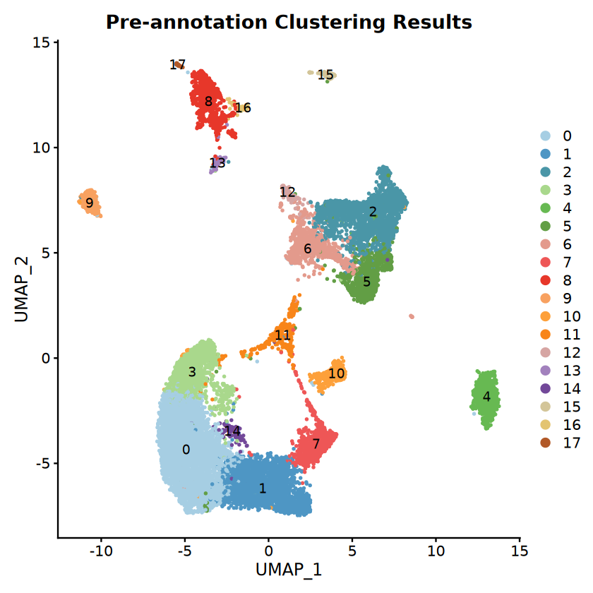
初始数据可视化

创建基本可视化以在注释前了解数据集结构。

# 基于聚类数量的自适应离散颜色
n_clusters <- length(table(seurat_obj[[resolution]]))
discrete_colors <- brewer.pal(min(n_clusters, 12), discrete_colors_name)
if (n_clusters > 12) {
    discrete_colors <- colorRampPalette(discrete_colors)(n_clusters)
}

cat("\n=== Color Scheme Updated ===\n")
cat("Number of clusters detected:", n_clusters, "\n")
cat("Discrete colors generated:", length(discrete_colors), "\n")

# 设置此可视化的绘图大小
options(repr.plot.width = 7, repr.plot.height = 7)

# 创建展示具有自适应颜色的聚类的 UMAP 图
p_clusters <- DimPlot(seurat_obj, 
                     reduction = "umap", 
                     group.by = resolution, 
                     label = TRUE, 
                     pt.size = 0.5, 
                     cols = discrete_colors) +
    ggtitle("Pre-annotation Clustering Results")

# 显示绘图
print(p_clusters)

# 保存绘图
ggsave(filename = file.path(output_path, "Step1_clusters_UMAP.pdf"), 
       plot = p_clusters, 
       width = 10, 
       height = 8, 
       dpi = 300)

cat("Initial clustering plot saved to:", file.path(output_path, "Step1_clusters_UMAP.pdf"), "\n")

output

=== Color Scheme Updated ===
Number of clusters detected: 18
Discrete colors generated: 18
Initial clustering plot saved to: /home/demo-seekgene-com/workspace/project/demo-seekgene-com/CellAnnotation/result/Step1_clusters_UMAP.pdf

使用 SingleR 进行自动注释

加载参考数据集

解析并加载指定的参考数据集以进行自动注释。

# 参考数据集缓存目录
cache_dir <- "/jp_envs/SingleR"

# 从参数解析参考数据集（支持逗号分隔值）
ref_datasets <- trimws(unlist(strsplit(reference_datasets, ",")))

# 基于物种验证参考数据集
if (species == "human") {
    valid_refs <- c("HumanPrimaryCellAtlas", "BlueprintEncode", "DatabaseImmuneCellExpression", "MonacoImmune", "NovershternHematopoietic")
} else if (species == "mouse") {
    valid_refs <- c("MouseRNAseq", "ImmGen")
} else {
    stop("Species must be either 'human' or 'mouse'")
}

# 检查指定的数据集是否有效
invalid_refs <- ref_datasets[!ref_datasets %in% valid_refs]
if (length(invalid_refs) > 0) {
    cat("Warning: Invalid reference datasets for", species, ":", paste(invalid_refs, collapse = ", "), "\n")
    cat("Valid options:", paste(valid_refs, collapse = ", "), "\n")
    ref_datasets <- ref_datasets[ref_datasets %in% valid_refs]
}

if (length(ref_datasets) == 0) {
    stop("No valid reference datasets specified")
}

cat("=== Loading Reference Datasets ===\n")
cat("Species:", species, "\n")
cat("Reference datasets:", paste(ref_datasets, collapse = ", "), "\n")

# 加载参考数据集
loaded_refs <- list()

for (ref_name in ref_datasets) {
    ref_path <- file.path(cache_dir, paste0(ref_name, ".rds"))
    
    if (file.exists(ref_path)) {
        cat("Loading reference dataset:", ref_name, "\n")
        ref_data <- readRDS(ref_path)
        loaded_refs[[ref_name]] <- ref_data
        
        # 显示参考数据集信息
        col_data <- colData(ref_data)
        if ("label.main" %in% colnames(col_data)) {
            cat("  - Number of cell types:", length(unique(col_data$label.main)), "\n")
            cat("  - Number of samples:", ncol(ref_data), "\n")
        }
    } else {
        cat("Warning: Reference dataset file not found:", ref_path, "\n")
        # 如果未缓存，尝试从 celldx 下载
        tryCatch({
            if (ref_name == "HumanPrimaryCellAtlas") {
                ref_data <- HumanPrimaryCellAtlasData()
            } else if (ref_name == "BlueprintEncode") {
                ref_data <- BlueprintEncodeData()
            } else if (ref_name == "DatabaseImmuneCellExpression") {
                ref_data <- DatabaseImmuneCellExpressionData()
            } else if (ref_name == "MonacoImmuneData") {
                ref_data <- MonacoImmuneData()
            } else if (ref_name == "MouseRNAseq") {
                ref_data <- MouseRNAseqData()
            } else if (ref_name == "ImmGen") {
                ref_data <- ImmGenData()
            }
            loaded_refs[[ref_name]] <- ref_data
            cat("Downloaded reference dataset:", ref_name, "\n")
        }, error = function(e) {
            cat("Error loading", ref_name, ":", e$message, "\n")
        })
    }
}

cat("Successfully loaded", length(loaded_refs), "reference dataset(s)\n")

output

=== Loading Reference Datasets ===
Species: human
Reference datasets: HumanPrimaryCellAtlas, BlueprintEncode
Loading reference dataset: HumanPrimaryCellAtlas
- Number of cell types: 36
- Number of samples: 713
Loading reference dataset: BlueprintEncode
- Number of cell types: 25
- Number of samples: 259
Successfully loaded 2 reference dataset(s)

运行 SingleR 注释

使用加载的参考数据集执行 SingleR 自动细胞类型注释。

if (length(loaded_refs) > 0) {
    cat("=== Running SingleR Annotation ===\n")
    
    # 提取表达矩阵
    expression_matrix <- GetAssayData(seurat_obj, assay = "RNA", slot = "data")
    
    # 存储 SingleR 结果
    singler_results <- list()
    
    # 对每个参考数据集运行 SingleR
    for (ref_name in names(loaded_refs)) {
        cat("正在运行 SingleR，参考数据集：", ref_name, "\n")
        
        ref_data <- loaded_refs[[ref_name]]
        
        cluster_vector <- seurat_obj[[resolution]][, 1]
        names(cluster_vector) <- rownames(seurat_obj[[resolution]])

        # 运行 SingleR 注释
        result <- SingleR(
            test = expression_matrix,
            ref = ref_data,
            labels = ref_data[[reference_label]],
            clusters = cluster_vector
        )
        
        singler_results[[ref_name]] <- result
        
        # 将聚类级别的注释添加到 Seurat 对象
        cluster_vector <- seurat_obj[[resolution]][, 1]
        names(cluster_vector) <- rownames(seurat_obj[[resolution]])
        cluster_annotations <- result$labels[match(cluster_vector, rownames(result))]
        seurat_obj@meta.data[[paste0("SingleR_", ref_name)]] <- cluster_annotations
        
        # 添加注释评分
        cluster_scores <- result$scores[match(cluster_vector, rownames(result)), ]
        max_scores <- apply(cluster_scores, 1, max, na.rm = TRUE)
        seurat_obj@meta.data[[paste0("SingleR_score_", ref_name)]] <- max_scores[match(cluster_vector, rownames(result))]
        
        cat("已完成注释，使用参考数据集：", ref_name, "\n")
        cat("识别出的细胞类型：", paste(unique(result$labels), collapse = ", "), "\n\n")
    }
    
    cat("=== SingleR 注释完成 ===\n")
} else {
    cat("错误：未加载参考数据集。无法继续 SingleR 注释。\n")
}

output

=== Running SingleR Annotation ===
Running SingleR with reference: HumanPrimaryCellAtlas
Completed annotation with HumanPrimaryCellAtlas
Identified cell types: T_cells, Monocyte, NK_cell, Macrophage, DC, B_cell, Neutrophils, Fibroblasts

Running SingleR with reference: BlueprintEncode
Completed annotation with BlueprintEncode
Identified cell types: CD8+ T-cells, Monocytes, HSC, Macrophages, NK cells, B-cells, Neutrophils, DC, Fibroblasts

=== SingleR Annotation Complete ===

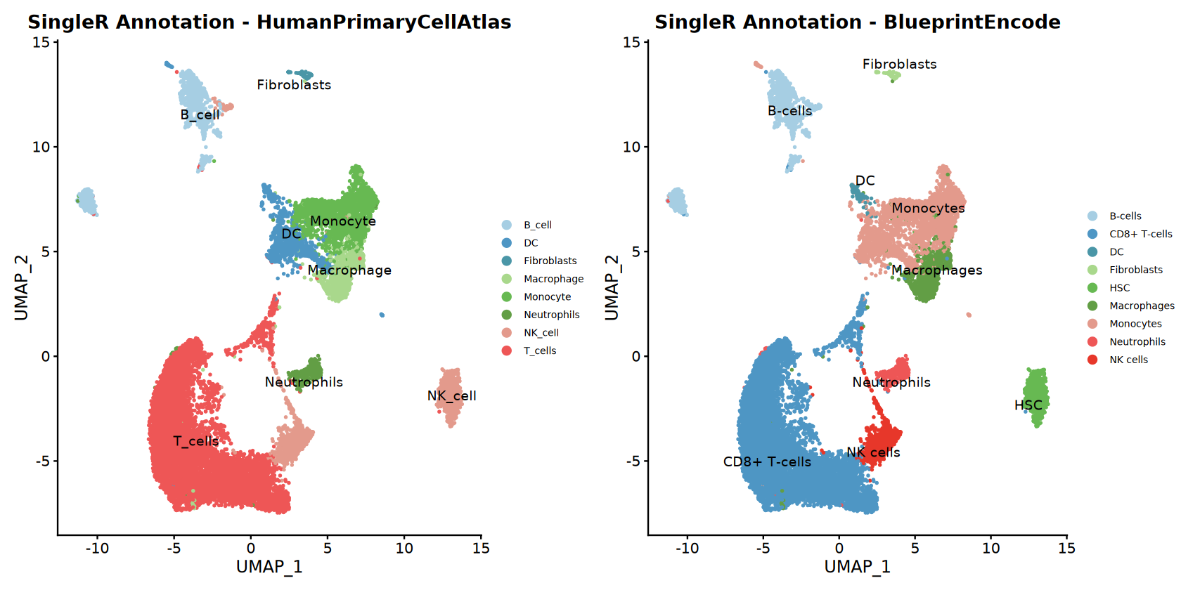
可视化 SingleR 结果

创建 SingleR 注释结果的综合可视化并展示。

if (exists("singler_results") && length(singler_results) > 0) {
    cat("=== Creating SingleR Annotation Visualizations ===\n")
    
    # 为每个参考数据集创建绘图
    singler_plots <- list()
    
    for (ref_name in names(singler_results)) {
        # 按 SingleR 注释着色的 UMAP 图
        p_singler <- DimPlot(seurat_obj, 
                            reduction = "umap", 
                            group.by = paste0("SingleR_", ref_name),
                            label = TRUE, 
                            pt.size = 0.5, 
                            cols = discrete_colors,
                            repel = TRUE) +
            ggtitle(paste("SingleR Annotation -", ref_name)) +
            theme(legend.text = element_text(size = 8),
                  plot.title = element_text(hjust = 0.5))
        
        singler_plots[[ref_name]] <- p_singler
        
        # 显示注释统计信息
        cat("\nAnnotation results for", ref_name, ":\n")
        annotation_table <- table(seurat_obj@meta.data[[paste0("SingleR_", ref_name)]])
        print(annotation_table)
        cat("\n")
    }
    
    # 如果有多个参考数据集，创建组合绘图
    if (length(singler_plots) > 0) {
        # 为组合绘图设置更大的尺寸
        options(repr.plot.width = 14, repr.plot.height = 7)
        
        combined_singler <- plot_grid(plotlist = singler_plots, ncol = 2)
        
        # 显示组合绘图
        print(combined_singler)
        
        ggsave(filename = file.path(output_path, "Step2_SingleR_UMAP.pdf"), 
               plot = combined_singler, 
               width = 16, 
               height = 12, 
               dpi = 300)
        
        cat("Saved combined SingleR plot\n")
    }
    
} else {
    cat("No SingleR results available for visualization\n")
}

output

=== Creating SingleR Annotation Visualizations ===

Annotation results for HumanPrimaryCellAtlas :

B_cell DC Fibroblasts Macrophage Monocyte Neutrophils
1370 1047 87 892 2243 411
NK_cell T_cells
1897 8977

Annotation results for BlueprintEncode :

B-cells CD8+ T-cells DC Fibroblasts HSC Macrophages
1448 8977 146 87 1014 892
Monocytes Neutrophils NK cells
3144 411 805

Saved combined SingleR plot

手动细胞类型注释

定义标记基因

使用标记基因执行手动细胞类型注释。

cat("=== 正在定义标记基因系统 ===\n")

# 定义物种特异性标记基因
if (species == "human") {
    cell_systems <- list(
        # 淋巴系统标记
        Lymphoid = list(
            B_cells = c("CD79A", "CD79B", "MS4A1"),
            Plasma_cells = c("JCHAIN", "MZB1", "IGHG1"),
            T_cells = c("CD3D", "CD3E", "CD3G", "CD2"),
            NK_cells = c("NKG7", "GNLY", "KLRF1", "KLRD1")
        ),
        
        # 髓系系统标记
        Myeloid = list(
            Monocytes = c("LYZ", "CTSS", "CD14", "FCGR3A"),
            Macrophages = c("CD68", "C1QA", "CD163", "CCL3", "VCAN"),
            DCs = c("CD74", "HLA-DPB1", "HLA-DPA1", "CD1C", "FCER1A", "CST3"),
            pDCs = c("LILRA4", "CLEC4C", "PLXNA4"),
            Granulocytes = c("ELANE", "MPO"),
            Neutrophils = c("S100A9", "S100A8", "FCGR3B", "CXCL8", "CSF3R"),
            Mast_cells = c("CPA3", "ENPP3", "HDC", "GATA2"),
            Megakaryocytes = c("PPBP", "PF4"),
            Erythrocytes = c("HBG1", "HBA1", "HBB")
        ),
    
        # 基质系统标记
        Stroma = list(
            Epithelial_cells = c("EPCAM", "KRT5", "KRT18"),
            Endothelial_cells = c("PECAM1", "ICAM2", "CLDN5", "CDH5", "PCDH17"),
            Fibroblasts = c("DCN", "COL1A2", "COL1A1"),
            Proliferating_cells = c("TOP2A", "MKI67")
        )
    )
    
} else if (species == "mouse") {
    # 小鼠特异性标记
    cell_systems <- list(
        Lymphoid = list(
            B_cells = c("Cd79a", "Cd79b", "Ms4a1", "Cd19"),
            Plasma_cells = c("Igha", "Jchain", "Iglv1"),
            T_cells = c("Cd3d", "Cd3e", "Cd3g"),
            NK_cells = c("Nkg7", "Icos", "Gzmb", "Prf1", "Klre1", "Gzma")
        ),
        
        Myeloid = list(
            Monocytes = c("Lyz2", "Cd14", "Csf1r", "Ctss"),
            Macrophages = c("Mrc1", "Arg1", "Cd163", "Cd68", "Adgre1"),
            DCs = c("Cd74", "H2-Aa", "H2-Ab1", "H2-Eb1", "Cd209a"),
            pDCs = c("Bst2", "Tcf4", "Irf8", "Siglech"),
            Granulocytes = c("Ngp", "Camp"),
            Neutrophils = c("S100a8", "S100a9", "Retnlg", "Csf3r"),
            Mast_cells = c("Cpa3"),
            Megakaryocytes = c("Pf4", "Ppbp"),
            Erythrocytes = c("Hba-a2", "Hbb-bs", "Hba-a1")
        ),
        
        Stroma = list(
            Epithelial_cells = c("Epcam", "Clcn3", "Cldn10", "Cldn3", "Krt7", "Krt8"),
            Endothelial_cells = c("Pecam1", "Cdh5", "Cldn5"),
            Fibroblasts = c("Col1a1", "Col1a2", "Dcn"),
            Proliferating_cells = c("Top2a", "Mki67")
        )
    )

} else {
    stop("Only mouse and human can do this analysis.")
}

# Output system information
for (system_name in names(cell_systems)) {
    cat(sprintf("%s system: %d cell types\n", 
                system_name,
                length(cell_systems[[system_name]])))
}

cat("\nMarker gene systems defined successfully\n")

output

=== Defining Marker Gene Systems ===
Lymphoid system: 4 cell types
Myeloid system: 9 cell types
Stroma system: 4 cell types

Marker gene systems defined successfully

创建绘图和评分函数

用于绘制标记基因并生成点图、热图、小提琴图和特征图的函数。

# 定义细胞系统的综合分析函数
analyze_cell_system <- function(seurat_obj, groups, markers, system_name, create_heatmap = TRUE, create_violin = TRUE, create_feature = TRUE, create_scoring = TRUE, print_plot = TRUE, step = "Step3") {
    cat(sprintf("\n=== %s 系统分析 ===\n", system_name))
    
    # 获取可用基因
    all_genes <- unlist(markers)
    available_genes <- all_genes[all_genes %in% rownames(seurat_obj)]
    
    if (length(available_genes) == 0) {
        cat(sprintf("警告：未找到 %s 系统的标记基因\n", system_name))
        return(seurat_obj)
    }
    
    cat(sprintf("找到 %d/%d 个标记基因\n", length(available_genes), length(all_genes)))
    
    # 1. 创建带有标记和基因集名称的点图 
    cat("正在创建带有标记和基因集名称的点图...\n")
    dotplot_width <- if(tolower(system_name) %in% c("all")) 20 else 20
    dotplot_height <- if(tolower(system_name) %in% c("all")) 10 else 8
    options(repr.plot.width = dotplot_width, repr.plot.height = dotplot_height)
    
    # 创建与可用基因完全匹配的基因集标签
    gene_labels <- c()
    ordered_genes <- c()
    
    for (cell_type in names(markers)) {
        genes_in_data <- markers[[cell_type]][markers[[cell_type]] %in% rownames(seurat_obj)]
        if (length(genes_in_data) > 0) {
            ordered_genes <- c(ordered_genes, genes_in_data)
            gene_labels <- c(gene_labels, rep(cell_type, length(genes_in_data)))
        }
    }
    
    # 使用排序后的基因以确保持致性
    if (length(ordered_genes) > 0) {
        dotplot <- DotPlot(seurat_obj, 
                          features = markers,
                          group.by = groups) +
            scale_color_gradientn(colors = continuous_colors) +
            theme(axis.text.x = element_text(angle = 45, hjust = 1, size = 9),
                  axis.text.y = element_text(size = 10),
                  plot.title = element_text(hjust = 0.5),
                  plot.margin = margin(t = 20, r = 10, b = 50, l = 10)) +
            ggtitle(sprintf("%s 系统标记 - 点图", system_name))
        
        if (print_plot) {
            print(dotplot)
        }
        
        # 保存点图
        filename <- sprintf("%s_%s_dotplot.pdf", step, tolower(gsub("[^A-Za-z0-9]", "_", system_name)))
        ggsave(filename = file.path(output_path, filename), 
               plot = dotplot, width = dotplot_width, height = dotplot_height, dpi = 300)
        
        cat(sprintf("点图已保存：%s\n", filename))
    } else {
        cat("没有可用于点图的基因\n")
    }
    
    # 2. Create heatmap
    if (create_heatmap && length(available_genes) > 0) {
        cat("正在创建热图...\\n")
        
        # 设置热图尺寸
        heatmap_width <- if(tolower(system_name) %in% c("all")) 20 else 20
        heatmap_height <- if(tolower(system_name) %in% c("all")) 10 else 8
        options(repr.plot.width = heatmap_width, repr.plot.height = heatmap_height)
        
        # 使用 DoHeatmap 创建热图
        tryCatch({
            # 如果细胞过多，进行降采样以提高热图性能
            max_cells_for_heatmap <- 1000
            if (ncol(seurat_obj) > max_cells_for_heatmap) {
                sample_cells <- sample(colnames(seurat_obj), max_cells_for_heatmap)
                heatmap_object <- subset(seurat_obj, cells = sample_cells)
            } else {
                heatmap_object <- seurat_obj
            }
            
            heatmap_plot <- DoHeatmap(heatmap_object, 
                                    features = available_genes,
                                    group.by = groups,
                                    size = 4,
                                    angle = 45,
                                    draw.lines = TRUE) +
                scale_fill_gradientn(colors = continuous_colors) +
                theme(axis.text.y = element_text(size = 8),
                      plot.title = element_text(hjust = 0.5)) +
                ggtitle(sprintf("%s 系统标记 - 热图", system_name))
            
            if (print_plot) {
                print(heatmap_plot)
            }
                            
            # 保存热图
            filename <- sprintf("%s_%s_heatmap.pdf", step, tolower(gsub("[^A-Za-z0-9]", "_", system_name)))
            ggsave(filename = file.path(output_path, filename), 
                   plot = heatmap_plot, width = heatmap_width, height = heatmap_height, dpi = 300)
            
            cat(sprintf("热图已保存：%s\\n", filename))
        }, error = function(e) {
            cat(sprintf("无法为 %s 创建热图：%s\\n", system_name, e$message))
        })
    } else {
        cat("没有可用于热图的基因\\n")
    }
    
    # 3. 创建堆叠小提琴图
    if (create_violin && length(available_genes) > 0) {
        cat("正在创建堆叠小提琴图...\n")
        violin_width <- if(tolower(system_name) %in% c("all")) 20 else 20
        violin_height <- if(tolower(system_name) %in% c("all")) 8 else 6
        options(repr.plot.width = violin_width, repr.plot.height = violin_height)
        
        # 基于基因数量的自适应离散颜色
        n_genes <- length(available_genes)
        genes_discrete_colors <- brewer.pal(min(n_genes, 12), discrete_colors_name)
        if (n_genes > 12) {
            genes_discrete_colors <- colorRampPalette(genes_discrete_colors)(n_genes)
        }
                
        violin_plot <- VlnPlot(seurat_obj, 
                              features = available_genes,
                              group.by = groups,
                              stack = TRUE,
                              flip = TRUE,
                              cols = genes_discrete_colors) +
            NoLegend() +
            ggtitle(sprintf("%s 系统标记 - 堆叠小提琴图", system_name)) +
            theme(plot.title = element_text(hjust = 0.5)) +
            theme(axis.text.x = element_text(angle = 0, hjust = 1))
        
        if (print_plot) {
        print(violin_plot)
        }
            
        filename <- sprintf("%s_%s_violin.pdf", step, tolower(gsub("[^A-Za-z0-9]", "_", system_name)))
        ggsave(filename = file.path(output_path, filename), 
               plot = violin_plot, width = violin_width, height = violin_height, dpi = 300)
        
        cat(sprintf("小提琴图已保存：%s\n", filename))
    }
    
    # 4. 创建前 6 个基因的特征图
    if (create_feature && length(available_genes) > 0) {
        cat("正在创建前 6 个基因的特征图...\n")
        top6_genes <- available_genes[1:min(6, length(available_genes))]
        
        featureplot_width <- if(tolower(system_name) %in% c("all")) 20 else 20
        featureplot_height <- if(tolower(system_name) %in% c("all")) 20 else 20
        options(repr.plot.width = featureplot_width, repr.plot.height = featureplot_height)
        
        feature_plot <- FeaturePlot(seurat_obj, 
                                   features = top6_genes,
                                   ncol = 3,
                                   reduction = "umap",
                                   col = continuous_colors) +
            theme(plot.title = element_text(hjust = 0.5, size = 12))

        feature_plot <- feature_plot + plot_annotation(
            title = sprintf("%s 系统标记 - 特征图", system_name),
            theme = theme(plot.title = element_text(hjust = 0.5, size = 16, face = "bold"))
            )
        
        if (print_plot) {
            print(feature_plot)
        }
            
        filename <- sprintf("%s_%s_top6_featureplot.pdf", step, tolower(gsub("[^A-Za-z0-9]", "_", system_name)))
        ggsave(filename = file.path(output_path, filename), 
               plot = feature_plot, width = featureplot_width, height = featureplot_height, dpi = 300)
        
        cat(sprintf("特征图已保存：%s\n", filename))
    }
    
    # 5. 基因集评分与可视化
    if (create_scoring) {
        cat("正在计算基因集评分...\n")
        
        for (cell_type in names(markers)) {
            genes <- markers[[cell_type]]
            genes <- genes[genes %in% rownames(seurat_obj)]
            
            if (length(genes) > 0) {
                score_name <- sprintf("%s_%s_Score", system_name, cell_type)
                seurat_obj <- AddModuleScore(seurat_obj, 
                                            features = list(genes), 
                                            name = score_name,
                                            seed = 42)
                colnames(seurat_obj@meta.data)[ncol(seurat_obj@meta.data)] <- score_name
                cat(sprintf("已添加 %s 评分\n", cell_type))
            }
        }
        
        # 获取评分列
        score_pattern <- sprintf("%s_.*_Score", system_name)
        score_columns <- grep(score_pattern, colnames(seurat_obj@meta.data), value = TRUE)
        
        if (length(score_columns) > 0) {
            # 基因集评分点图
            cat("正在创建基因集评分点图...\n")
            score_dotplot_width <- if(tolower(system_name) %in% c("all")) 20 else 20
            score_dotplot_height <- if(tolower(system_name) %in% c("all")) 10 else 8
            options(repr.plot.width = score_dotplot_width, repr.plot.height = score_dotplot_height)
            score_dotplot <- DotPlot(seurat_obj, 
                              features = score_columns,
                              group.by = groups) +
                scale_color_gradientn(colors = continuous_colors) +
                theme(plot.title = element_text(hjust = 0.5, size = 10),
                    axis.text.x = element_text(angle = 45, hjust = 1, size = 9)) +
                ggtitle(sprintf("%s 系统模块评分 - 点图", system_name))

            if (print_plot) {
                print(score_dotplot)
            }
                
            filename <- sprintf("%s_%s_score_dotplot.pdf", step, tolower(gsub("[^A-Za-z0-9]", "_", system_name)))
            ggsave(filename = file.path(output_path, filename), 
                   plot = score_dotplot, width = score_dotplot_width, height = score_dotplot_height, dpi = 300)
            
            cat(sprintf("评分点图已保存：%s\n", filename))

            # 基因集评分热图
            cat("正在创建基因集评分热图...\n")
            score_heatmap_width <- if(tolower(system_name) %in% c("all")) 10 else 20
            score_heatmap_height <- if(tolower(system_name) %in% c("all")) 8 else 6           
            avg_score <- sapply(score_columns, function(sc) tapply(seurat_obj@meta.data[[sc]], seurat_obj@meta.data[[groups]], mean, na.rm = TRUE))
            avg_score <- t(avg_score) 

            score_heatmap <- pheatmap(
                avg_score,
                cluster_rows = FALSE,
                cluster_cols = FALSE,
                show_colnames = TRUE,
                show_rownames = TRUE,
                angle_col = 0,
                color = continuous_colors,
                cellwidth = 80,
                cellheight = 60,
                main = paste0(system_name, " 系统模块评分 - 热图")
            )

            filename <- sprintf("%s_%s_score_heatmap.pdf", step, tolower(gsub("[^A-Za-z0-9]", "_", system_name)))
            ggsave(filename = file.path(output_path, filename), 
                   plot = score_heatmap, width = score_heatmap_width, height = score_heatmap_height, dpi = 300)
            
            cat(sprintf("评分热图已保存：%s\n", filename))
            
            # 基因集评分小提琴图
            cat("正在创建基因集评分小提琴图...\n")
            score_violin_width <- if(tolower(system_name) %in% c("all")) 20 else 20
            score_violin_height <- if(tolower(system_name) %in% c("all")) 24 else 14
            ncol_val <- if(tolower(system_name) %in% c("all")) 3 else 2
            options(repr.plot.width = score_violin_width, repr.plot.height = score_violin_height)
            
            score_violin <- VlnPlot(seurat_obj, 
                                   features = score_columns,
                                   group.by = groups,
                                   ncol = ncol_val,
                                   pt.size = 0,
                                   cols = discrete_colors) &
                theme(plot.title = element_text(hjust = 0.5, size = 10))

            score_violin <- score_violin + plot_annotation(
                title = sprintf("%s 系统模块评分 - 小提琴图", system_name),
                theme = theme(plot.title = element_text(hjust = 0.5, size = 16, face = "bold"))
                )
            
            if (print_plot) {
                print(score_violin)
            }
                                
            filename <- sprintf("%s_%s_score_violin.pdf", step, tolower(gsub("[^A-Za-z0-9]", "_", system_name)))
            ggsave(filename = file.path(output_path, filename), 
                   plot = score_violin, width = score_violin_width, height = score_violin_height, dpi = 300)
            
            cat(sprintf("评分小提琴图已保存：%s\n", filename))
            
            # 基因集评分特征图
            cat("正在创建基因集评分特征图...\n")
            score_featureplot_width <- if(tolower(system_name) %in% c("all")) 20 else 20
            score_featureplot_height <- if(tolower(system_name) %in% c("all")) 24 else 14
            options(repr.plot.width = score_featureplot_width, repr.plot.height = score_featureplot_height)
            
            score_feature <- FeaturePlot(seurat_obj, 
                                        features = score_columns,
                                        ncol = ncol_val,
                                        reduction = "umap",
                                        cols = continuous_colors) &
                theme(plot.title = element_text(hjust = 0.5, size = 10))

            score_feature <- score_feature + plot_annotation(
                title = sprintf("%s 系统模块评分 - 特征图", system_name),
                theme = theme(plot.title = element_text(hjust = 0.5, size = 16, face = "bold"))
                )
            
            if (print_plot) {
                print(score_feature)
            }
                                
            filename <- sprintf("%s_%s_score_featureplot.pdf", step, tolower(gsub("[^A-Za-z0-9]", "_", system_name)))
            ggsave(filename = file.path(output_path, filename), 
                   plot = score_feature, width = score_featureplot_width, height = score_featureplot_height, dpi = 300)
            
            cat(sprintf("评分特征图已保存：%s\n", filename))
        }
    }
    
    cat(sprintf("%s 系统分析完成\n", system_name))
    return(seurat_obj)
}

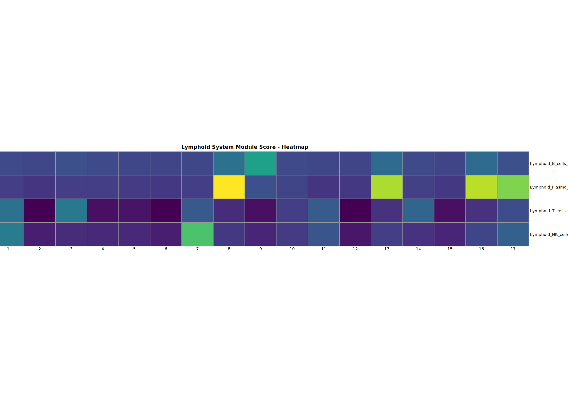
cat("分析函数定义成功\n")

output

Analysis function defined successfully

淋巴系统分析

B 细胞、浆细胞、T 细胞和 NK 细胞的综合分析，包括点图、堆叠小提琴图、热图、前 6 个基因特征图和基因集评分。

# 淋巴系统分析
cat("=== 开始淋巴系统分析 ===\n")

seurat_obj <- analyze_cell_system(
    seurat_obj = seurat_obj,
    groups = resolution,
    markers = cell_systems$Lymphoid,
    system_name = "Lymphoid",
    create_heatmap = TRUE,
    create_violin = TRUE,
    create_feature = TRUE,
    create_scoring = TRUE,
    print_plot = FALSE,
    step = "Step3"
)

cat("淋巴系统分析完成\n")

output

=== Starting Lymphoid System Analysis ===

=== Lymphoid System Analysis ===
Found 14/14 marker genes
Creating dotplot with marker and gene set names...n

Warning message:
“The \`facets\` argument of \`facet_grid()\` is deprecated as of ggplot2 2.2.0.
ℹ Please use the \`rows\` argument instead.
ℹ The deprecated feature was likely used in the Seurat package.
Please report the issue at .”
Scale for colour is already present.
Adding another scale for colour, which will replace the existing scale.

Dotplot saved: Step3_lymphoid_dotplot.pdf
Creating heatmap...

Warning message in DoHeatmap(heatmap_object, features = available_genes, group.by = groups, :
“The following features were omitted as they were not found in the scale.data slot for the RNA assay: KLRF1, CD2, CD3G, CD3E, CD3D, CD79B”
Scale for fill is already present.
Adding another scale for fill, which will replace the existing scale.

Heatmap saved: Step3_lymphoid_heatmap.pdf\
Creating stacked violin plot...n Violin plot saved: Step3_lymphoid_violin.pdf
Creating top 6 genes featureplot...n Feature plot saved: Step3_lymphoid_top6_featureplot.pdf
Calculating gene set scores...n Added B_cells score
Added Plasma_cells score
Added T_cells score
Added NK_cells score
Creating gene set scoring dotplot...n

Scale for colour is already present.
Adding another scale for colour, which will replace the existing scale.

Score dotplot saved: Step3_lymphoid_score_dotplot.pdf
Creating gene set scoring heatmap...n Score heatmap saved: Step3_lymphoid_score_heatmap.pdf
Creating gene set scoring violin plot...n Score violin plot saved: Step3_lymphoid_score_violin.pdf
Creating gene set scoring featureplot...n Score feature plot saved: Step3_lymphoid_score_featureplot.pdf
Lymphoid system analysis completed
Lymphoid system analysis completed

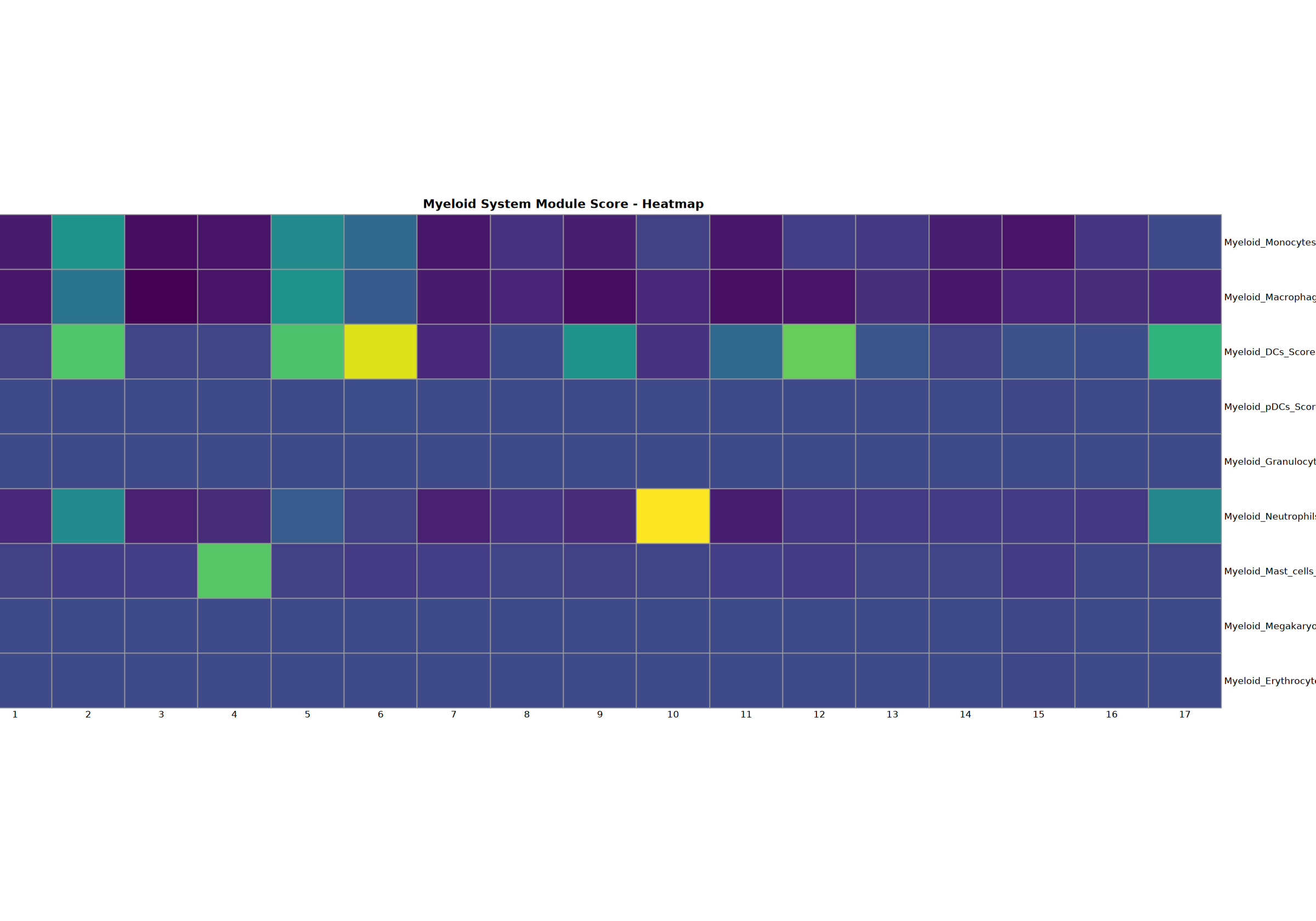
髓系系统分析

对单核细胞、巨噬细胞、DC、pDC、粒细胞、中性粒细胞、肥大细胞、巨核细胞和红细胞进行综合分析。

# 髓系系统分析
cat("=== 开始髓系系统分析 ===\n")

seurat_obj <- analyze_cell_system(
    seurat_obj = seurat_obj,
    groups = resolution,
    markers = cell_systems$Myeloid,
    system_name = "Myeloid",
    create_heatmap = TRUE,
    create_violin = TRUE,
    create_feature = TRUE,
    create_scoring = TRUE,
    print_plot = FALSE,
    step = "Step3"
)

cat("髓系系统分析完成\n")

output

=== Starting Myeloid System Analysis ===

=== Myeloid System Analysis ===
Found 33/34 marker genes
Creating dotplot with marker and gene set names...n

Warning message in FetchData.Seurat(object = object, vars = features, cells = cells):
“The following requested variables were not found: HBG1”
Scale for colour is already present.
Adding another scale for colour, which will replace the existing scale.

Dotplot saved: Step3_myeloid_dotplot.pdf
Creating heatmap...

Warning message in DoHeatmap(heatmap_object, features = available_genes, group.by = groups, :
“The following features were omitted as they were not found in the scale.data slot for the RNA assay: HBA1, PF4, CSF3R, MPO, ELANE, PLXNA4, CLEC4C, HLA-DPA1, HLA-DPB1, CD74, CTSS”
Scale for fill is already present.
Adding another scale for fill, which will replace the existing scale.

Heatmap saved: Step3_myeloid_heatmap.pdf\
Creating stacked violin plot...n Violin plot saved: Step3_myeloid_violin.pdf
Creating top 6 genes featureplot...n Feature plot saved: Step3_myeloid_top6_featureplot.pdf
Calculating gene set scores...n Added Monocytes score
Added Macrophages score
Added DCs score
Added pDCs score
Added Granulocytes score
Added Neutrophils score
Added Mast_cells score
Added Megakaryocytes score
Added Erythrocytes score
Creating gene set scoring dotplot...n

Scale for colour is already present.
Adding another scale for colour, which will replace the existing scale.

Score dotplot saved: Step3_myeloid_score_dotplot.pdf
Creating gene set scoring heatmap...n Score heatmap saved: Step3_myeloid_score_heatmap.pdf
Creating gene set scoring violin plot...n Score violin plot saved: Step3_myeloid_score_violin.pdf
Creating gene set scoring featureplot...n Score feature plot saved: Step3_myeloid_score_featureplot.pdf
Myeloid system analysis completed
Myeloid system analysis completed

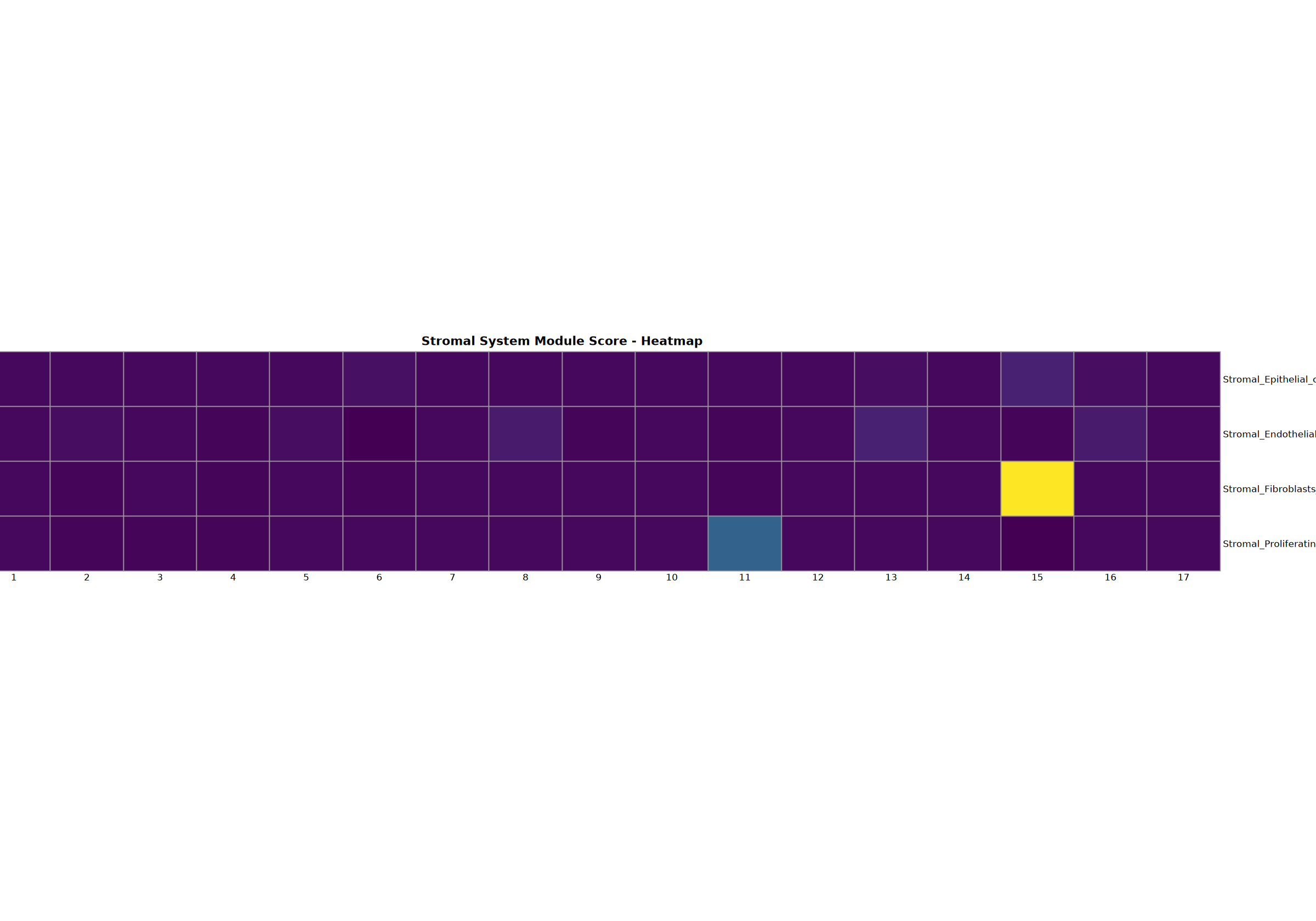
基质系统分析

上皮细胞、内皮细胞、成纤维细胞和增殖细胞的分析。

# 基质系统分析（根据要求仅绘制点图）
cat("=== 开始基质系统分析 ===\n")

seurat_obj <- analyze_cell_system(
    seurat_obj = seurat_obj,
    groups = resolution,
    markers = cell_systems$Stroma,
    system_name = "Stromal",
    create_heatmap = TRUE,
    create_violin = TRUE,
    create_feature = TRUE,
    create_scoring = TRUE,
    print_plot = FALSE,
    step = "Step3"
)

cat("基质系统分析完成\n")

output

=== Starting Stromal System Analysis ===

=== Stromal System Analysis ===
Found 12/13 marker genes
Creating dotplot with marker and gene set names...n

Warning message in FetchData.Seurat(object = object, vars = features, cells = cells):
“The following requested variables were not found: CDH5”
Scale for colour is already present.
Adding another scale for colour, which will replace the existing scale.

Dotplot saved: Step3_stromal_dotplot.pdf
Creating heatmap...

Warning message in DoHeatmap(heatmap_object, features = available_genes, group.by = groups, :
“The following features were omitted as they were not found in the scale.data slot for the RNA assay: PCDH17, ICAM2, PECAM1”
Scale for fill is already present.
Adding another scale for fill, which will replace the existing scale.

Heatmap saved: Step3_stromal_heatmap.pdf\
Creating stacked violin plot...n Violin plot saved: Step3_stromal_violin.pdf
Creating top 6 genes featureplot...n Feature plot saved: Step3_stromal_top6_featureplot.pdf
Calculating gene set scores...n Added Epithelial_cells score
Added Endothelial_cells score
Added Fibroblasts score
Added Proliferating_cells score
Creating gene set scoring dotplot...n

Scale for colour is already present.
Adding another scale for colour, which will replace the existing scale.

Score dotplot saved: Step3_stromal_score_dotplot.pdf
Creating gene set scoring heatmap...n Score heatmap saved: Step3_stromal_score_heatmap.pdf
Creating gene set scoring violin plot...n Score violin plot saved: Step3_stromal_score_violin.pdf
Creating gene set scoring featureplot...n Score feature plot saved: Step3_stromal_score_featureplot.pdf
Stromal system analysis completed
Stromal system analysis completed

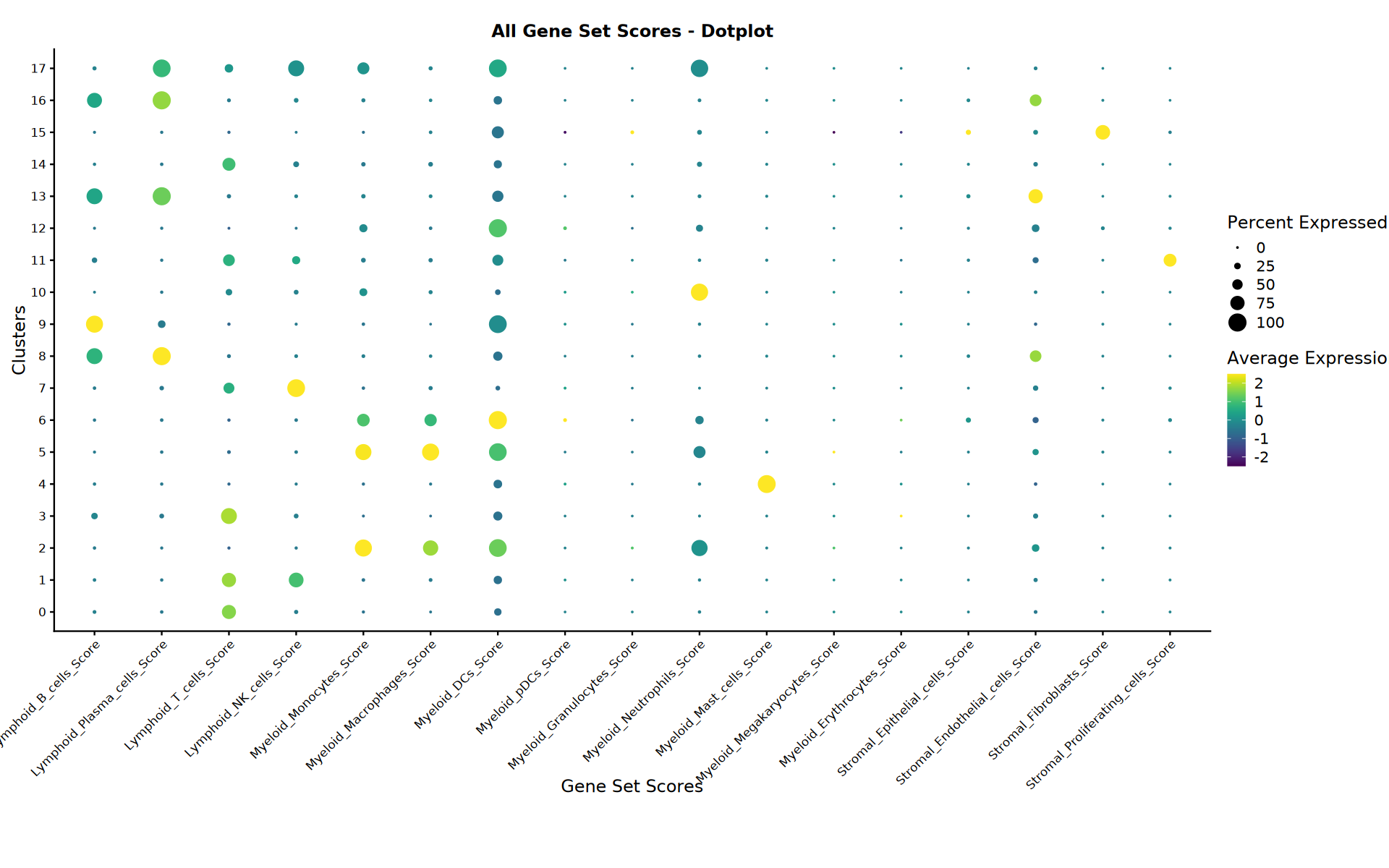
分析总结

显示已完成分析和生成文件的总结。

# === 所有评分点图 ===
cat("=== 正在创建所有评分点图 ===")

# 获取所有评分列
all_scores <- grep(".*_.*_Score$", colnames(seurat_obj@meta.data), value = TRUE)

if (length(all_scores) > 0) {
    cat(sprintf("发现 %d 个用于可视化的基因集评分", length(all_scores)))
    
    # 设置绘图尺寸
    options(repr.plot.width = 16, repr.plot.height = 10)
    
    # 创建组合评分点图
    tryCatch({
        scores_dotplot <- DotPlot(seurat_obj, 
                                features = all_scores,
                                group.by = resolution) +
            scale_color_gradientn(colors = continuous_colors) +
            theme(axis.text.x = element_text(angle = 45, hjust = 1, size = 10),
                  axis.text.y = element_text(size = 10),
                  plot.title = element_text(hjust = 0.5, size = 14),
                  plot.margin = margin(t = 20, r = 10, b = 60, l = 10)) +
            ggtitle("所有基因集评分 - 点图") +
            labs(x = "基因集评分", y = "聚类")
        
        print(scores_dotplot)
        
        # 保存所有评分点图
        ggsave(filename = file.path(output_path, "Step3_All_Scores_dotplot.pdf"), 
               plot = scores_dotplot, width = 20, height = 15, dpi = 300)
        
        cat("所有评分点图已保存: Step3_All_Scores_dotplot.pdf")
    }, error = function(e) {
        cat(sprintf("无法创建所有评分点图: %s", e))
    })
} else {
    cat("未找到用于可视化的基因集评分")
}

output

=== Creating All Scores Dotplot ===Found 17 gene set scores for visualization

Scale for colour is already present.
Adding another scale for colour, which will replace the existing scale.

All scores dotplot saved: Step3_All_Scores_dotplot.pdf

cat("=== 手动注释分析总结 ===\n")

# 统计生成的评分
all_scores <- grep(".*_.*_Score$", colnames(seurat_obj@meta.data), value = TRUE)
cat(sprintf("生成了 %d 个基因集评分\n", length(all_scores)))

if (length(all_scores) > 0) {
    cat("基因集评分:\n")
    for (score in all_scores) {
        cat("  -", score, "\n")
    }
}

# 列出生成的文件
cat("\n生成的可视化文件:\n")
pdf_files <- list.files(output_path, pattern = "\\.pdf$", full.names = FALSE)
annotation_files <- pdf_files[grepl("(lymphoid|myeloid|stromal)", pdf_files, ignore.case = TRUE)]
for (file in annotation_files) {
    cat("  -", file, "\n")
}

cat("\n分析成功完成!\n")

output

=== Manual Annotation Analysis Summary ===
Generated 17 gene set scores
Gene set scores:
- Lymphoid_B_cells_Score
- Lymphoid_Plasma_cells_Score
- Lymphoid_T_cells_Score
- Lymphoid_NK_cells_Score
- Myeloid_Monocytes_Score
- Myeloid_Macrophages_Score
- Myeloid_DCs_Score
- Myeloid_pDCs_Score
- Myeloid_Granulocytes_Score
- Myeloid_Neutrophils_Score
- Myeloid_Mast_cells_Score
- Myeloid_Megakaryocytes_Score
- Myeloid_Erythrocytes_Score
- Stromal_Epithelial_cells_Score
- Stromal_Endothelial_cells_Score
- Stromal_Fibroblasts_Score
- Stromal_Proliferating_cells_Score

Generated visualization files:
- Step3_lymphoid_dotplot.pdf
- Step3_lymphoid_heatmap.pdf
- Step3_lymphoid_score_dotplot.pdf
- Step3_lymphoid_score_featureplot.pdf
- Step3_lymphoid_score_heatmap.pdf
- Step3_lymphoid_score_violin.pdf
- Step3_lymphoid_top6_featureplot.pdf
- Step3_lymphoid_violin.pdf
- Step3_myeloid_dotplot.pdf
- Step3_myeloid_heatmap.pdf
- Step3_myeloid_score_dotplot.pdf
- Step3_myeloid_score_featureplot.pdf
- Step3_myeloid_score_heatmap.pdf
- Step3_myeloid_score_violin.pdf
- Step3_myeloid_top6_featureplot.pdf
- Step3_myeloid_violin.pdf
- Step3_stromal_dotplot.pdf
- Step3_stromal_heatmap.pdf
- Step3_stromal_score_dotplot.pdf
- Step3_stromal_score_featureplot.pdf
- Step3_stromal_score_heatmap.pdf
- Step3_stromal_score_violin.pdf
- Step3_stromal_top6_featureplot.pdf
- Step3_stromal_violin.pdf

Analysis completed successfully!

保存 RDS 结果

保存手动注释的 Seurat 对象。

cat("=== 正在保存最终结果 ===\n")

# 保存注释后的 Seurat 对象
annotated_seurat_path <- file.path(output_path, "Step3_Cell_Annotation.rds")
saveRDS(seurat_obj, annotated_seurat_path)
cat("已保存注释后的 Seurat 对象至:", annotated_seurat_path, "\n")

output

=== Saving Final Results ===
Saved annotated Seurat object to: /home/demo-seekgene-com/workspace/project/demo-seekgene-com/CellAnnotation/result/Step3_Cell_Annotation.rds

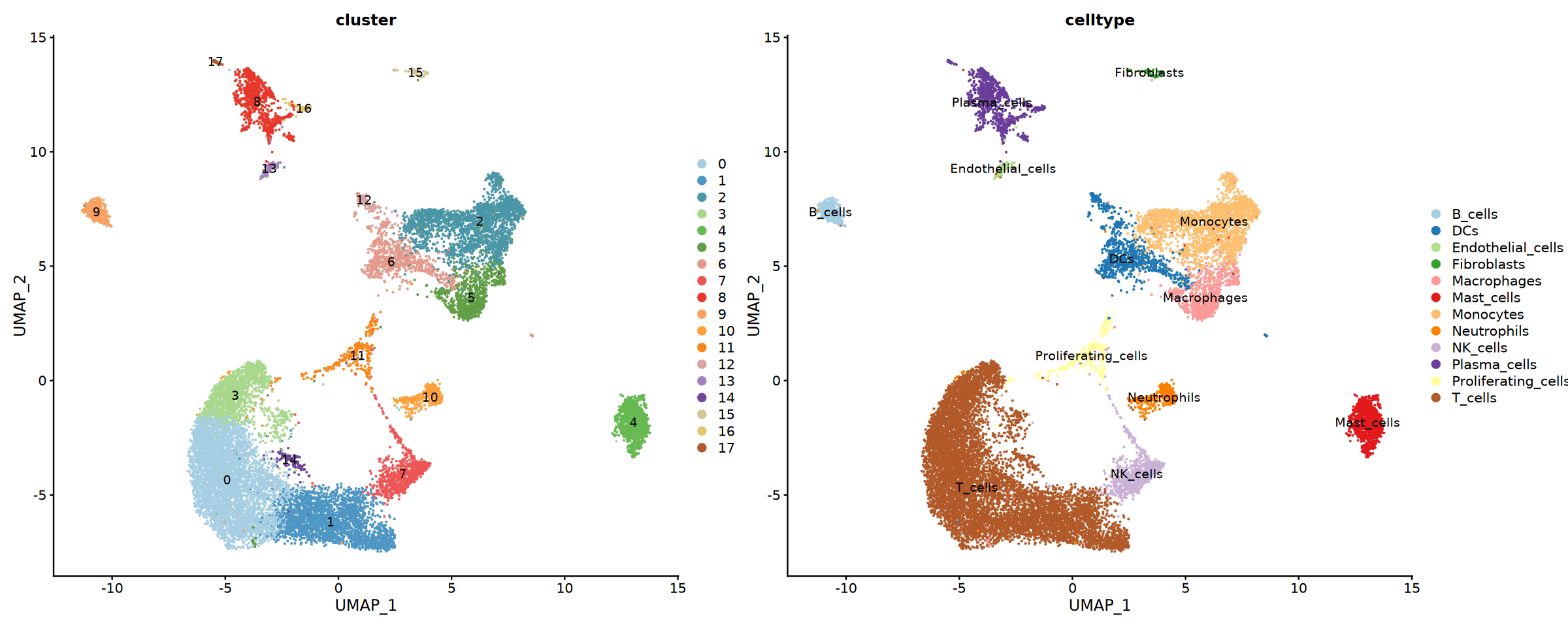
最终细胞类型注释

参数配置

读取 RDS 文件，添加细胞类型名称，并绘制最终细胞注释结果的 UMAP 图。

cat("=== 第四步：最终细胞类型注释 ===\n")

# 执行最终细胞注释
Final_Cell_Annotation <- TRUE

# 定义注释后的 Seurat 对象路径
annotated_seurat_path <- file.path(output_path, "Step3_Cell_Annotation.rds")

# 细胞注释信息的标签命名
anno_label <- "celltype"

# 定义一个命名向量，将每个聚类 ID 映射到具有生物学意义的细胞类型标签。
cat("正在添加细胞类型...\n")
cluster_to_celltype <- c(
    "0" = "T_cells",
    "1" = "T_cells", 
    "2" = "Monocytes",
    "3" = "T_cells",
    "4" = "Mast_cells",
    "5" = "Macrophages",
    "6" = "DCs",
    "7" = "NK_cells",
    "8" = "Plasma_cells",
    "9" = "B_cells",
    "10" = "Neutrophils",
    "11" = "Proliferating_cells",
    "12" = "DCs",
    "13" = "Endothelial_cells",
    "14" = "T_cells",
    "15" = "Fibroblasts",
    "16" = "Plasma_cells",
    "17" = "Plasma_cells"
)

# 为每种细胞类型定义标记基因列表。
cat("正在添加细胞类型标记...\n")
cell_system_markers <- list(
    B_cells = c("CD79A", "CD79B", "MS4A1"),
    DCs = c("CD74", "HLA-DPB1", "HLA-DPA1", "CD1C", "FCER1A", "CST3"),
    Endothelial_cells = c("PECAM1", "ICAM2", "CLDN5", "CDH5", "PCDH17"),
    Fibroblasts = c("DCN", "COL1A2", "COL1A1"),
    Macrophages = c("CD68", "C1QA", "CD163", "CCL3", "VCAN"),
    Mast_cells = c("CPA3", "ENPP3", "HDC", "GATA2"),
    Monocytes = c("LYZ", "CTSS", "CD14", "FCGR3A"),
    Neutrophils = c("S100A9", "S100A8", "FCGR3B", "CXCL8", "CSF3R"),
    NK_cells = c("NKG7", "GNLY", "KLRF1", "KLRD1"),
    Plasma_cells = c("JCHAIN", "MZB1", "IGHG1"),
    Proliferating_cells = c("TOP2A", "MKI67"),
    T_cells = c("CD3D", "CD3E", "CD3G", "CD2")
)

output

=== Step 4: Final Cell Type Annotation ===
Adding cell types...n Adding cell type markers...

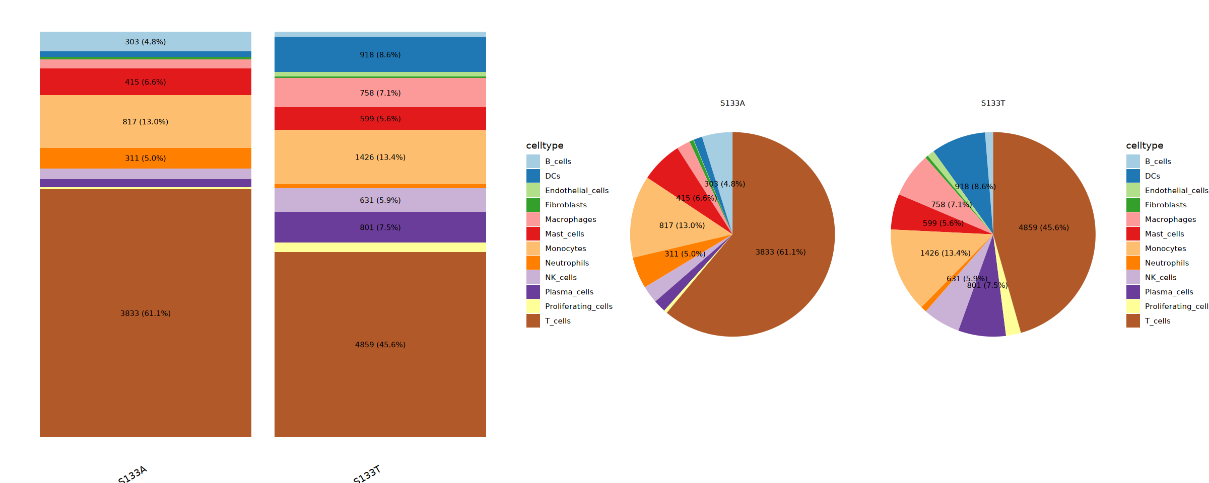
创建细胞类型比较函数

用于比较不同分组中细胞类型数量和比例的函数。

celltype_comp <- function(meta,
                          annotation_col = "celltype",
                          group = "sample",
                          plot_width = 20,
                          plot_height = 8,
                          label_min_prop = 0.03) {
  group_cols <- strsplit(group, ",")[[1]] |> trimws()

  old_opt <- options(repr.plot.width = plot_width, repr.plot.height = plot_height)

  df <- meta |>
    tidyr::unite("group_key", tidyselect::all_of(group_cols), sep = " | ", remove = FALSE) |>
    dplyr::count(group_key, annotation = .data[[annotation_col]], name = "n") |>
    dplyr::group_by(group_key) |>
    dplyr::mutate(prop = n / sum(n)) |>
    dplyr::ungroup() |>
    dplyr::mutate(label_text = ifelse(
      prop >= label_min_prop,
      paste0(n, " (", scales::percent(prop, accuracy = 0.1), ")"),
      NA
    ))

  p_bar <- ggplot(df, aes(x = group_key, y = prop, fill = annotation)) +
    geom_col() +
    geom_text(aes(label = label_text),
              position = position_stack(vjust = 0.5),
              color = "black", size = 3, na.rm = TRUE) +
    scale_y_continuous(labels = scales::label_percent(accuracy = 1)) +
    scale_fill_manual(values = celltype_discrete_colors) +
    labs(x = "分组", y = "比例", fill = annotation_col) +
    theme_void() +
    theme(axis.text.x = element_text(angle = 30, hjust = 1))

  p_pie <- ggplot(df, aes(x = "", y = prop, fill = annotation)) +
    scale_fill_manual(values = celltype_discrete_colors) +
    geom_col(width = 1) +
    geom_text(aes(label = label_text),
              position = position_stack(vjust = 0.5),
              color = "black", size = 3, na.rm = TRUE) +
    coord_polar(theta = "y") +
    facet_wrap(~ group_key) +
    labs(fill = annotation_col) +
    theme_void()

    return(p_bar + p_pie)
}

可视化最终细胞注释结果

绘制细胞类型的 UMAP 图，以及不同分组中细胞比例的堆叠柱状图和饼图。

if (Final_Cell_Annotation & file.exists(annotated_seurat_path)) {

    cat("正在加载注释后的 Seurat 对象...\n")
    # 加载步骤3保存的 Seurat 对象
    seurat_final <- readRDS(annotated_seurat_path)
    
    # 从指定分辨率提取聚类标识
    cluster_vector <- seurat_final[[resolution]][, 1]
    names(cluster_vector) <- rownames(seurat_final[[resolution]])
    
    # 根据聚类标识为每个细胞分配细胞类型标签
    seurat_final[[anno_label]] <- cluster_to_celltype[as.character(cluster_vector)]
    
    # 显示聚类与分配的细胞类型的对照表
    table(seurat_final@meta.data[[resolution]], seurat_final@meta.data[[anno_label]])
    
    cat("正在创建最终 UMAP 可视化图...\n")
    
    # 设置绘图尺寸（宽度和高度）
    options(repr.plot.width = 20, repr.plot.height = 8)
    
    # 创建按聚类着色的 UMAP 图
    umap_clusters <- DimPlot(seurat_final, 
                           reduction = "umap", 
                           group.by = resolution, 
                           cols = discrete_colors,
                           label = TRUE, 
                           label.size = 4) +
        ggtitle("聚类") +
        theme(plot.title = element_text(hjust = 0.5, size = 14))

    n_celltypes <- length(table(seurat_final[[anno_label]]))
    celltype_discrete_colors <- brewer.pal(min(n_celltypes, 12), discrete_colors_name)
    if (n_celltypes > 12) {
        celltype_discrete_colors <- colorRampPalette(discrete_colors)(n_celltypes)
    } 

    # 创建按分配的细胞类型着色的 UMAP 图
    umap_celltypes <- DimPlot(seurat_final, 
                            reduction = "umap", 
                            group.by = anno_label, 
                            cols = celltype_discrete_colors,
                            label = TRUE, 
                            label.size = 4) +
        ggtitle(anno_label) +
        theme(plot.title = element_text(hjust = 0.5, size = 14))
    
    # 将两个图并排组合
    combined_umap <- umap_clusters + umap_celltypes
    
    # 显示组合图
    print(combined_umap)
    
    # 将组合 UMAP 图保存为 PDF 文件
    ggsave(filename = file.path(output_path, "Step4_Final_Cell_Annotation_UMAP.pdf"), 
           plot = combined_umap, width = 20, height = 8, dpi = 300)
    
    cat("最终 UMAP 图已保存：Step4_Final_Cell_Annotation_UMAP.pdf\n")
    
    cat("正在创建最终细胞类型比例可视化图...\n")

    combined_prop <- celltype_comp(seurat_final@meta.data,annotation_col = anno_label, group = "sample")

    print(combined_prop)

    # 将细胞类型比例图保存为 PDF 文件
    ggsave(filename = file.path(output_path, "Step4_Final_Cell_Type_Proportion.pdf"), 
           plot = combined_prop, width = 20, height = 8, dpi = 300)
    
    cat("最终比例图已保存：Step4_Final_Cell_Type_Proportion.pdf\n")
    
    # 保存完全注释的 Seurat 对象用于下游分析
    final_annotated_path <- file.path(output_path, "Step4_Final_Cell_Annotation.rds")
    saveRDS(seurat_final, final_annotated_path)
    
    cat("最终注释的 Seurat 对象已保存：", final_annotated_path, "\n")
        
}

output

Loading annotated Seurat object...n Creating final UMAP visualization...n Final UMAP saved: Step4_Final_Cell_Annotation_UMAP.pdf
Creating final cell type proportion visualization...

Final Proportion saved: Step4_Final_Cell_Type_Proportion.pdf
Final annotated Seurat object saved: /home/demo-seekgene-com/workspace/project/demo-seekgene-com/CellAnnotation/result/Step4_Final_Cell_Annotation.rds

全系统分析

对最终细胞注释结果进行分析。

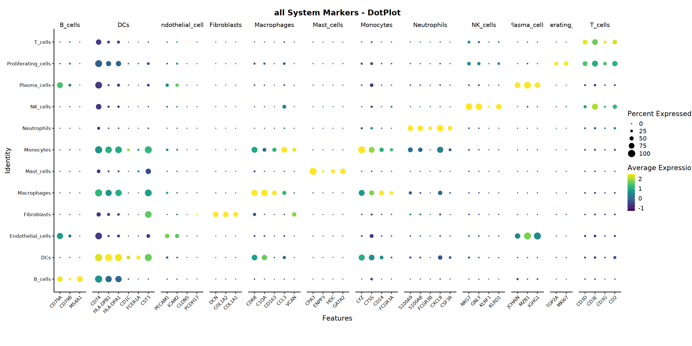
# 运行自定义函数 `analyze_cell_system` 为标记基因生成各种图表
if (Final_Cell_Annotation & file.exists(annotated_seurat_path)) {
    cat("正在为每个细胞系统生成标记基因可视化...\n")
    seurat_obj <- analyze_cell_system(
        seurat_obj = seurat_final,
        groups = anno_label,
        markers = cell_system_markers,
        system_name = "all",
        create_heatmap = TRUE,
        create_violin = TRUE,  
        create_feature = TRUE,  
        create_scoring = TRUE,  
        print_plot = TRUE,
        step = "Step4"      
    )
}

cat("\n=== 分析完成 ===\n")
cat("所有结果已保存至:", output_path, "\n")
cat("生成的文件总数:", length(list.files(output_path)), "\n")

output

Generating marker gene visualizations for each cell system...n
=== all System Analysis ===
Found 47/48 marker genes
Creating dotplot with marker and gene set names...n

Warning message in FetchData.Seurat(object = object, vars = features, cells = cells):
“The following requested variables were not found: CDH5”
Scale for colour is already present.
Adding another scale for colour, which will replace the existing scale.

Dotplot saved: Step4_all_dotplot.pdf
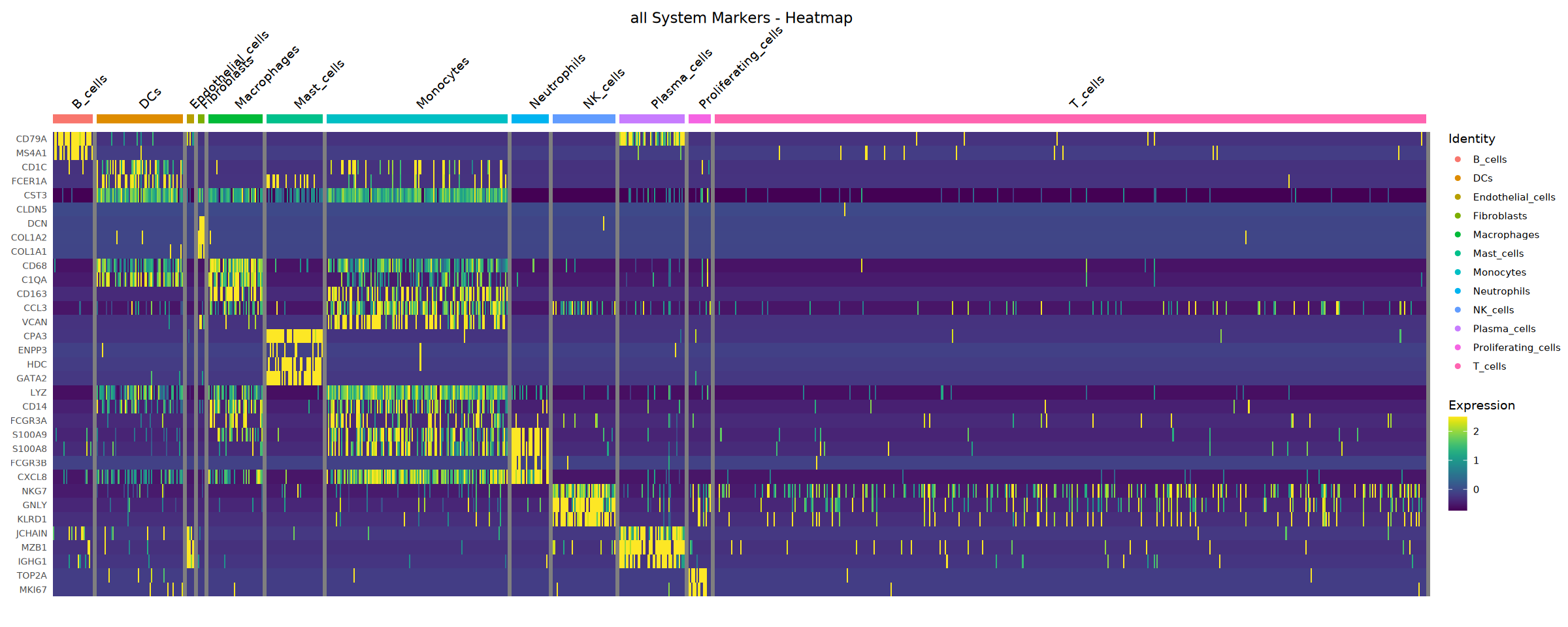
Creating heatmap...

Warning message in DoHeatmap(heatmap_object, features = available_genes, group.by = groups, :
“The following features were omitted as they were not found in the scale.data slot for the RNA assay: CD2, CD3G, CD3E, CD3D, KLRF1, CSF3R, CTSS, PCDH17, ICAM2, PECAM1, HLA-DPA1, HLA-DPB1, CD74, CD79B”
Scale for fill is already present.
Adding another scale for fill, which will replace the existing scale.

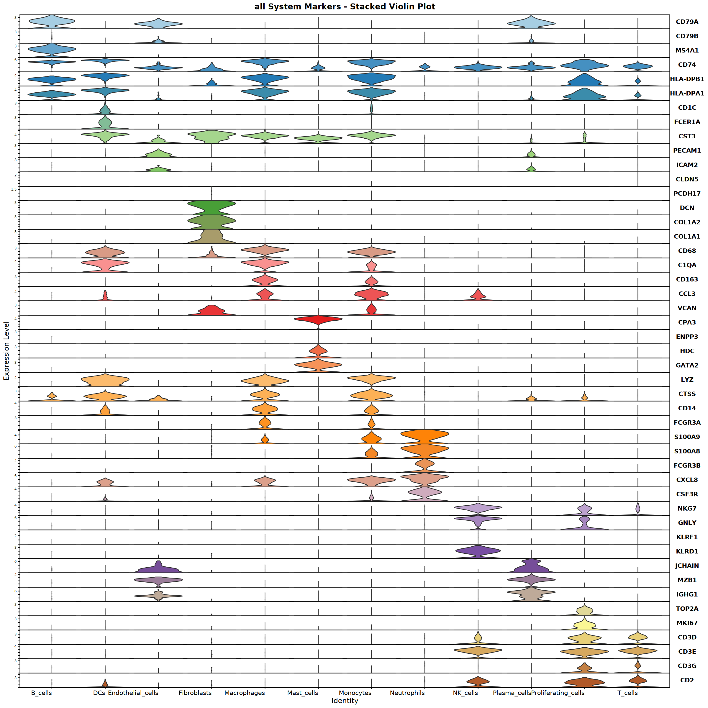
Heatmap saved: Step4_all_heatmap.pdf\nCreating stacked violin plot...

Violin plot saved: Step4_all_violin.pdf
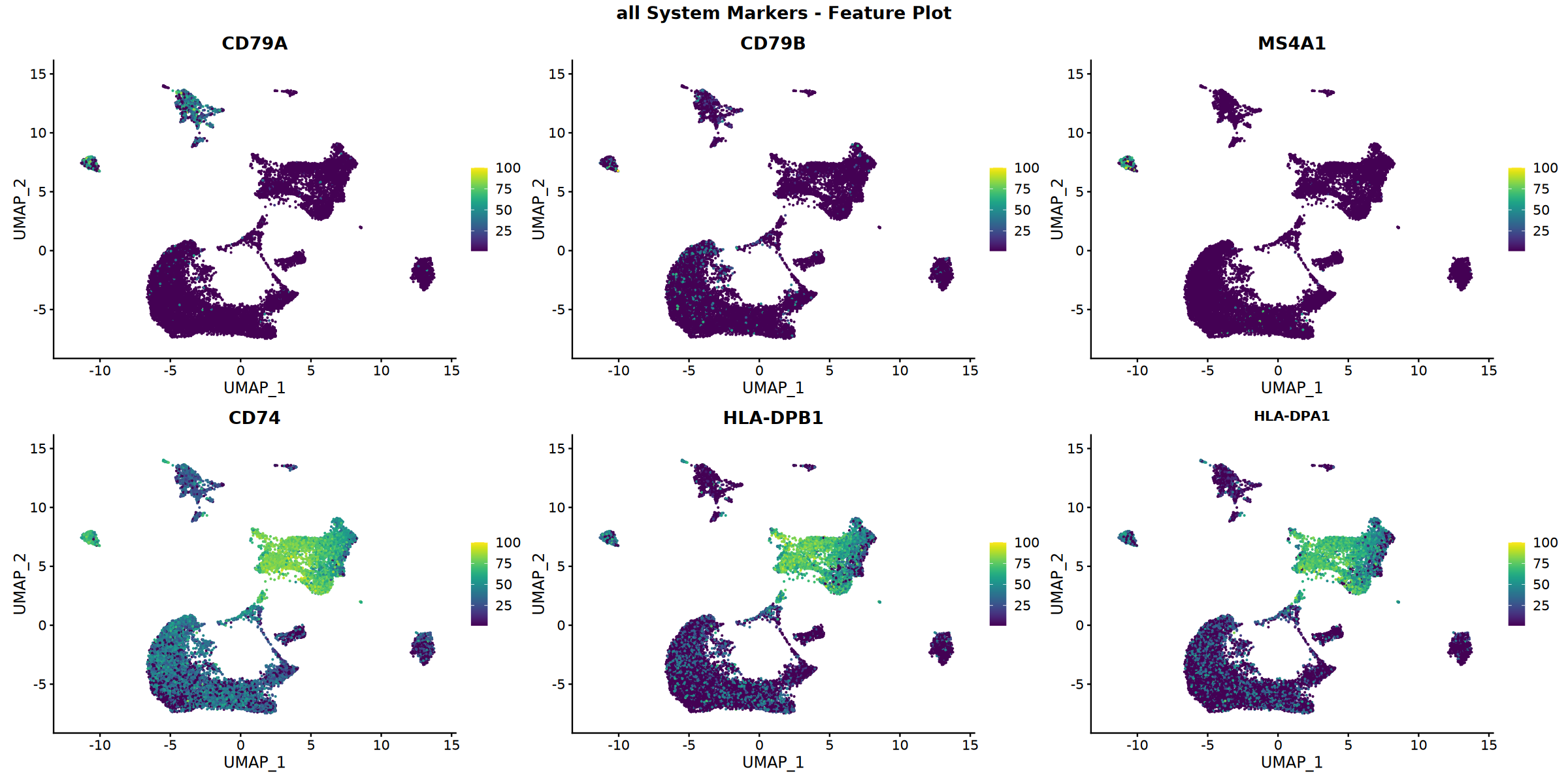
Creating top 6 genes featureplot...

Feature plot saved: Step4_all_top6_featureplot.pdf
Calculating gene set scores...
Added B_cells score
Added DCs score
Added Endothelial_cells score
Added Fibroblasts score
Added Macrophages score
Added Mast_cells score
Added Monocytes score
Added Neutrophils score
Added NK_cells score
Added Plasma_cells score
Added Proliferating_cells score
Added T_cells score
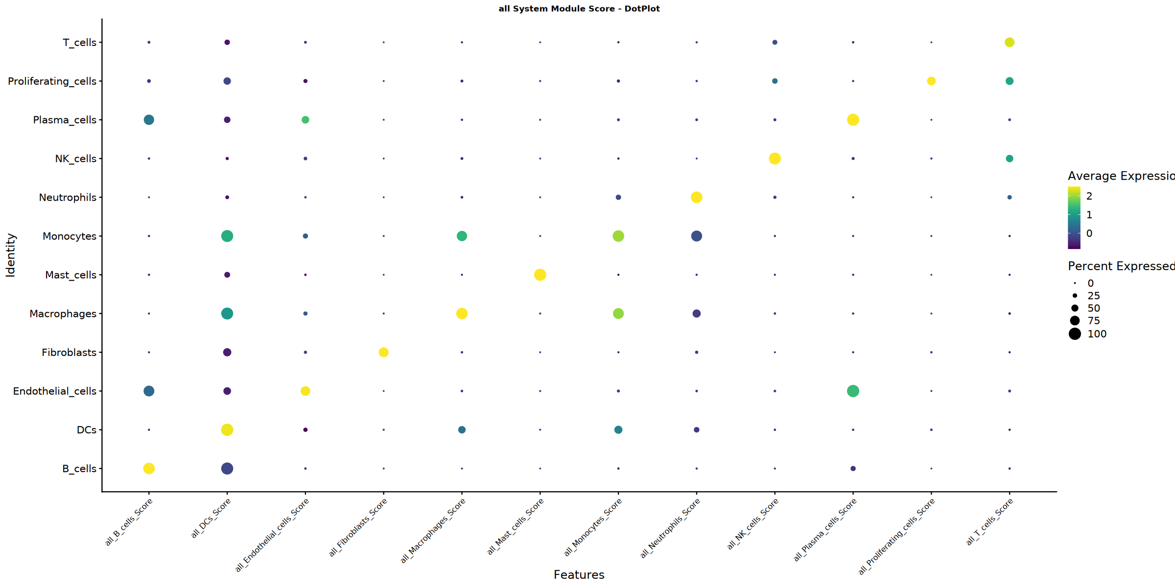
Creating gene set scoring dotplot...


[1m[22mScale for [32mcolour[39m is already present.
Adding another scale for [32mcolour[39m, which will replace the existing scale.

Score dotplot saved: Step4_all_score_dotplot.pdf
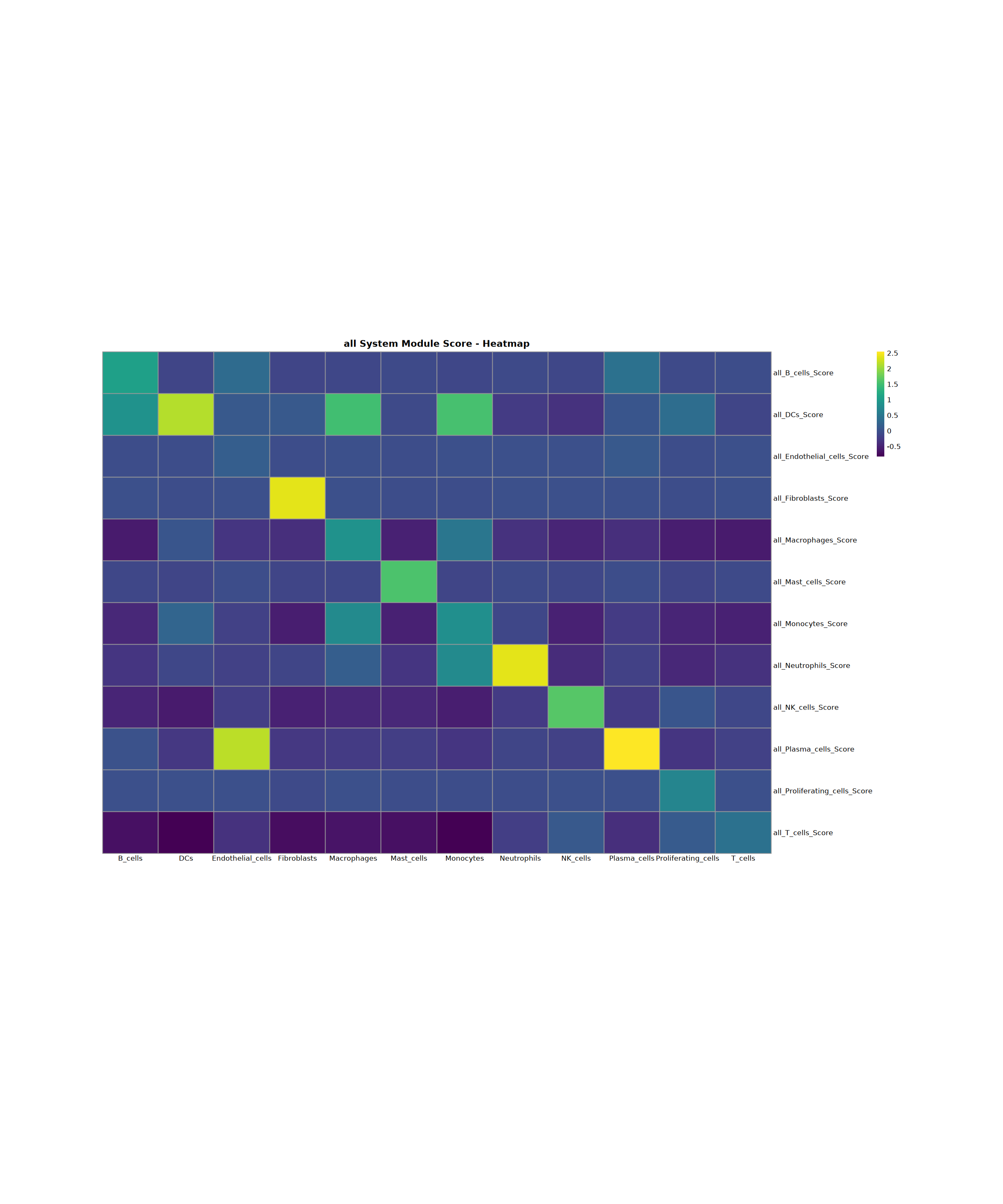
Creating gene set scoring heatmap...

Score heatmap saved: Step4_all_score_heatmap.pdf
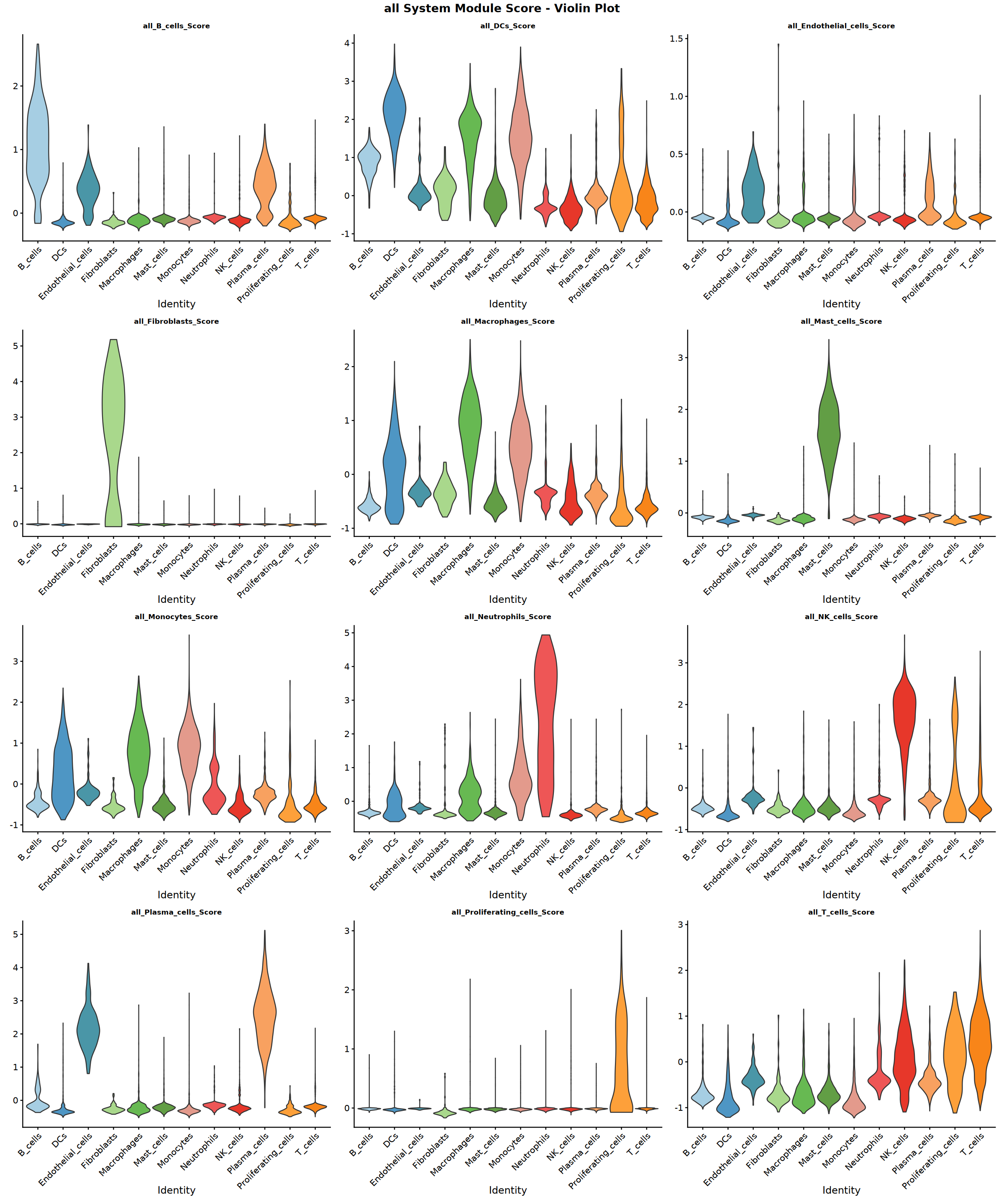
Creating gene set scoring violin plot...

Score violin plot saved: Step4_all_score_violin.pdf
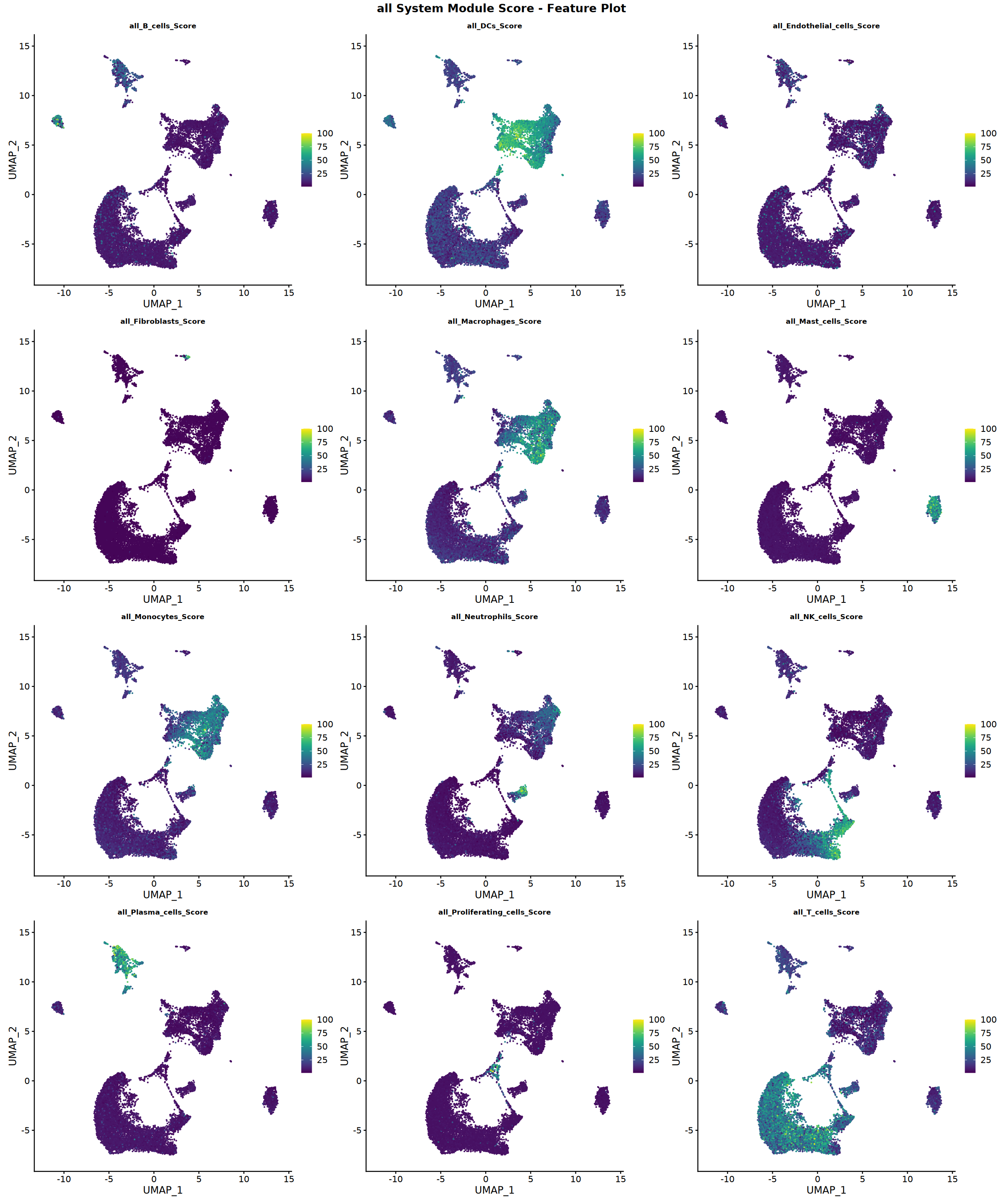
Creating gene set scoring featureplot...

Score feature plot saved: Step4_all_score_featureplot.pdf
all system analysis completed

=== Analysis Complete ===
All results saved to: /home/demo-seekgene-com/workspace/project/demo-seekgene-com/CellAnnotation/result 
Total files generated: 39

模板信息

模板发布日期: 2025年8月26日
最后更新: 2025年8月26日

联系方式: 有关本教程的问题、议题或建议，请通过 "智能咨询" 服务联系我们。

参考文献与引用

[1] Seurat Package: https://github.com/satijalab/seurat.

[2] SingleR: https://github.com/dviraran/SingleR. Liu X., Wu C., Pan L., et al. (2025). SeekSoul Online: A user-friendly bioinformatics platform focused on single-cell multi-omics analysis. The Innovation Life 3:100156. https://doi.org/10.59717/j.xinn-life.2025.100156

单细胞转录组细胞注释教程：基于 Marker 基因的类型识别 ​

细胞注释简介 ​

什么是细胞注释？ ​

SingleR 简介 ​

内核配置 ​

加载库与参数配置 ​

加载库 ​

配置分析参数 ​

综合细胞类型注释教程 ​

数据准备 ​

加载并检查 Seurat 对象 ​

初始数据可视化 ​

使用 SingleR 进行自动注释 ​

加载参考数据集 ​

运行 SingleR 注释 ​

可视化 SingleR 结果 ​

手动细胞类型注释 ​

定义标记基因 ​

创建绘图和评分函数 ​

淋巴系统分析 ​

髓系系统分析 ​

基质系统分析 ​

分析总结 ​

保存 RDS 结果 ​

最终细胞类型注释 ​

参数配置 ​

创建细胞类型比较函数 ​

可视化最终细胞注释结果 ​

全系统分析 ​

模板信息 ​

参考文献与引用 ​

单细胞转录组细胞注释教程：基于 Marker 基因的类型识别

细胞注释简介

什么是细胞注释？

SingleR 简介

内核配置

加载库与参数配置

加载库

配置分析参数

综合细胞类型注释教程

数据准备

加载并检查 Seurat 对象

初始数据可视化

使用 SingleR 进行自动注释

加载参考数据集

运行 SingleR 注释

可视化 SingleR 结果

手动细胞类型注释

定义标记基因

创建绘图和评分函数

淋巴系统分析

髓系系统分析

基质系统分析

分析总结

保存 RDS 结果

最终细胞类型注释

参数配置

创建细胞类型比较函数

可视化最终细胞注释结果

全系统分析

模板信息

参考文献与引用