拟时序相关基因筛选教程:探索基因表达随轨迹的动态变化
时长: 4 分钟
字数: 807 字
更新: 2026-02-28
阅读: 0 次
运行环境
R
##############################
# 选择jupyter脚本执行环境为 monocle2(R) #
##############################
加载依赖包
R
suppressMessages({
library(monocle)
library(Seurat)
library(dplyr)
library(tidyverse)
library(ggplot2)
library(ggsci)
})
读取分析结果
R
#读取monocle2的分析结果
monocle<-readRDS("demo_monocle2/output/monocle2/monocle_final.rds")
方法说明:拟时序自然样条
sm.ns 函数的作用是指定软件通过拟合自然样条曲线来处理基因表达值。自然样条是一种数学函数,它能够平滑地连接数据点,形成一条连续的曲线。
差异分析
R
diff_test_res = differentialGeneTest(monocle, fullModelFormulaStr = "~sm.ns(Pseudotime)")结果预览
R
#查看前5行
head(diff_test_res[,c("gene_short_name", "pval", "qval")])| gene_short_name | pval | qval | |
|---|---|---|---|
| <chr> | <dbl> | <dbl> | |
| AL627309.1 | AL627309.1 | 1.256879e-20 | 1.188652e-19 |
| AL627309.5 | AL627309.5 | 1.474717e-32 | 2.049121e-31 |
| AP006222.2 | AP006222.2 | 8.636056e-02 | 1.579091e-01 |
| AL732372.1 | AL732372.1 | 1.647113e-01 | 2.657367e-01 |
| LINC01409 | LINC01409 | 2.159786e-01 | 3.301703e-01 |
| FAM87B | FAM87B | 8.604796e-02 | 1.574697e-01 |
选择示例基因
R
#这里选取的基因作为demo测试(选取自己的目标基因进行替换)
marker_gene = c('LEPR','VCAM1','BGLAP','RUNX2','COL1A1','SPARC','NR4A1','NR4A2')
提取拟时相关基因
R
gene_time <- diff_test_res[marker_gene,] %>%
    na.omit() %>%
    pull(gene_short_name) %>%
    as.character()
绘制拟时序表达曲线
可以使用 plot_genes_in_pseudotime 函数来绘制这些基因的表达水平,这些基因的表达水平都随着分化过程(伪时间)显示出显著的变化。这个函数还提供了许多美化选项,你可以用来控制绘图的布局和外观。
R
# 绘制基因表达轨迹图
p = plot_genes_in_pseudotime(monocle[gene_time,],
                             color_by = "subtype",
                             ncol = 2)
p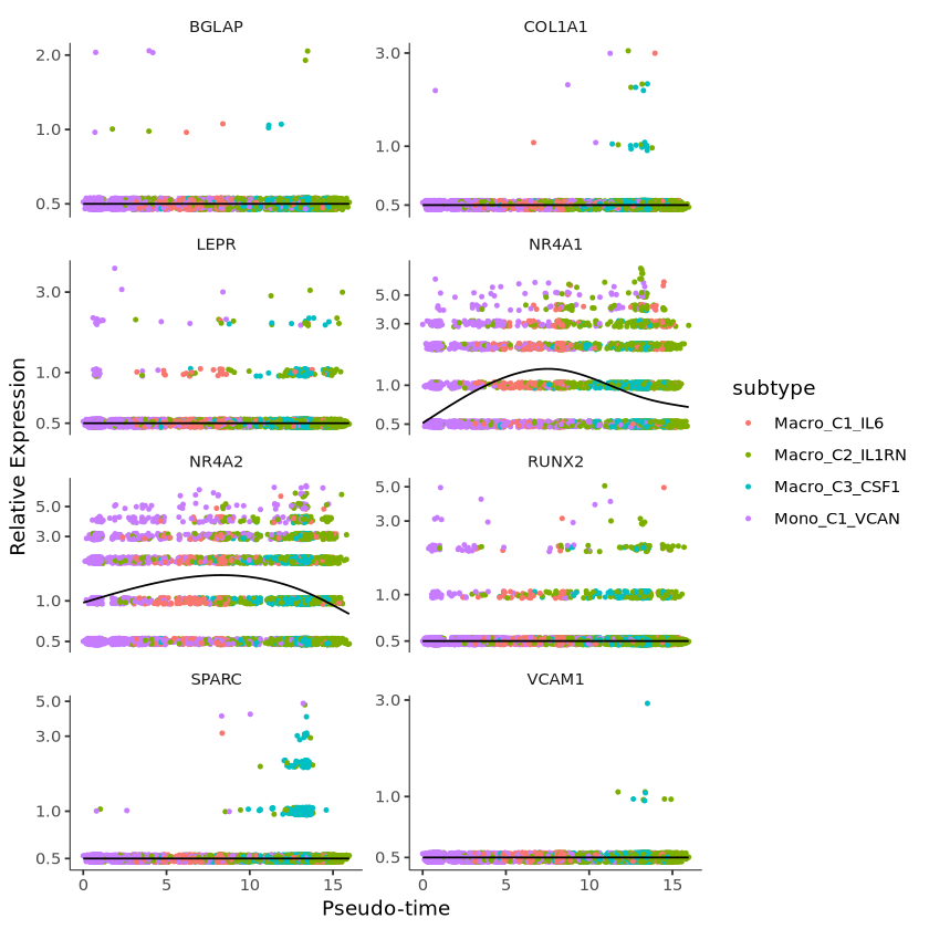
R
p1 = p +
  facet_wrap(~gene_short_name, scales = "free", ncol = 2) +
  theme(strip.text = element_text(size = 15),
        axis.text.x = element_text(size = 10),
        axis.text.y = element_text(size = 10))+
guides(color = guide_legend(title = "demo"))

p1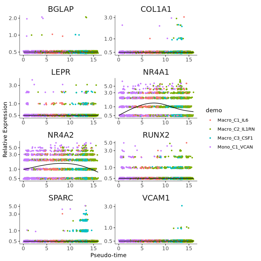
根据拟时表达模式对基因进行聚类
Monocle 提供了一种方便的方式来可视化所有与拟时序相关的基因。plot_pseudotime_heatmap 函数接收一个 CellDataSet 对象(通常只包含显著基因的一个子集),并像 plot_genes_in_pseudotime 一样生成平滑的表达曲线。然后,它对这些基因进行聚类,并使用 pheatmap 包进行绘制。这使得你可以可视化在拟时序上共同变化的基因模块。
R
#绘制热图
p2 = plot_pseudotime_heatmap(monocle[gene_time,],
                        num_cluster = 3,
                        show_rownames = T,
                        return_heatmap = T)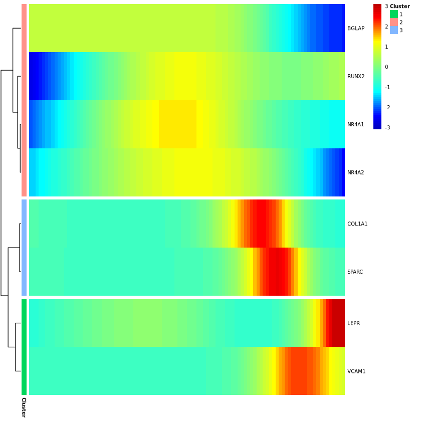
R
#保存图片
ggsave("plot.pdf", p1, width = 8, height = 12)
ggsave("heatmap.pdf", p2, width = 5, height = 6)