单细胞空间微环境解析：细胞 Niche 分析与聚类教程

作者: SeekGene

时长: 6 分钟

字数: 1.1k 字

更新: 2026-02-28

阅读: 0 次

空间转录组 分析指南 Notebooks 生态位分析

加载分析包

import numpy as np
import pandas as pd
import scanpy as sc
import seaborn as sns
from sklearn.neighbors import NearestNeighbors
from sklearn.cluster import MiniBatchKMeans
import matplotlib.pyplot as plt
from matplotlib.pyplot import rc_context
import stlearn as st

output

/PROJ2/FLOAT/jinwen/apps/miniconda3/envs/COMMOT/lib/python3.10/site-packages/stlearn/tools/microenv/cci/het.py:192: NumbaDeprecationWarning: The keyword argument 'nopython=False' was supplied. From Numba 0.59.0 the default is being changed to True and use of 'nopython=False' will raise a warning as the argument will have no effect. See https://numba.readthedocs.io/en/stable/reference/deprecation.html#deprecation-of-object-mode-fall-back-behaviour-when-using-jit for details.
@jit(parallel=True, nopython=False)

读取矩阵数据

• 分析前，需要将 input.rds 转化为三个矩阵文件，才能读取
• 分析前，需要注释好细胞类型

adata = sc.read_10x_mtx("filtered_feature_bc_matrix/")
spatial = pd.read_csv('filtered_feature_bc_matrix/cell_locations.tsv',sep="\t",index_col=0)
spatial = spatial.loc[:,("x","y")]
selected_rows = spatial.loc[spatial.index.isin(adata.obs_names)]
selected_rows.columns = ["imagecol","imagerow"]
selected_rows = selected_rows.reindex(adata.obs_names)
# 使用st.create_stlearn可以将表达，空间位置导入anndata对象；若还想要导入图片，添加参数image_path。SeekSpace技术中一个像素点的大小是约为0.265385微米，故scale=0.265385。
a = st.create_stlearn(count=adata.to_df(),spatial=selected_rows,library_id="N1", scale=0.265385,spot_diameter_fullres=10)
cluster_name = "celltype"
celltype = pd.read_csv("../../data/AY1748480899609/meta.tsv",index_col=0,sep = "\t")

celltype = celltype.loc[a.obs.index]
## meta_celltype_colums_name为原rds里metadata中细胞类型列名
meta_celltype_colums_name = "CellAnnotation"
a.obs[cluster_name] = celltype[meta_celltype_colums_name]
a.obs[cluster_name] = a.obs[cluster_name].astype('category')
#a = a[a.obs["celltype"].isin(["HSC","Fibroblasts"])]

#a.layers["raw_count"] = a.X
a.layers["counts"] = a.X
sc.pp.normalize_total(a, target_sum=1e4)
sc.pp.log1p(a)
sc.pp.calculate_qc_metrics(a, percent_top=None, log1p=False, inplace=True)

• Step 1: 使用半径搜索邻居
• Step 2: 处理邻居索引（按距离排序 + 排除自身）
• Step 3: 计算窗口和（处理稀疏区域）
• Step 4: 聚类邻域类型

def cell_neighbors(adata,column,radius=20,n_clusters=10):
    spatial_coords = adata.obsm['spatial']
    onehot_encoding = pd.get_dummies(adata.obs[column])
    cluster_cols = adata.obs[column].unique()
    values = onehot_encoding[cluster_cols].values
    nbrs = NearestNeighbors(radius=radius,metric='euclidean').fit(spatial_coords)
    distances,indices = nbrs.radius_neighbors(spatial_coords,return_distance=True)   
    sorted_indices = []
    for i in range(len(indices)):
        if len(indices[i]) == 0:
            sorted_indices.append(np.array([]))
            continue # 按距离排序并排除自身
        sorted_order = np.argsort(distances[i])
        neigh_indices = indices[i][sorted_order]
        mask = (neigh_indices != i)
        filtered_indices = neigh_indices[mask]
        sorted_indices.append(filtered_indices)
    def compute_window_sums(sorted_indices,values):
        windows = []
        for idx in range(len(sorted_indices)):
            neighbors = sorted_indices[idx]
            if len(neighbors) == 0: # 稀疏区域处理：使用自身类型填充
                window_sum = values[idx] # 自身类型
            else:
                window_sum = values[neighbors].sum(axis=0)
            # 归一化为比例分布
            window_sum_norm = window_sum / (window_sum.sum() + 1e-6) # 防止零除
            windows.append(window_sum_norm)
        return np.array(windows)
    windows = compute_window_sums(sorted_indices,values)
    
    km = MiniBatchKMeans(n_clusters=n_clusters, random_state=0)
    labels = km.fit_predict(windows)
    adata.obs[f'CNs_{n_clusters}'] = [f'CN{i}' for i in labels] # 可视化 Fold Change    
    k_centroids = km.cluster_centers_
    tissue_avgs = values.mean(axis=0)
    fc = np.log2((k_centroids + 1e-6) / (tissue_avgs + 1e-6)) # 避免零除
    fc_df = pd.DataFrame(fc,columns=cluster_cols)
    fc_df.index = [f'CN{i}' for i in range(n_clusters)]
    sns.set_style("white")
    g = sns.clustermap(fc_df,vmin=-2,vmax=2,cmap="vlag",row_cluster=False,col_cluster=True,linewidths=0.5,figsize=(6,6))
    g.ax_heatmap.tick_params(right=False,bottom=False)

    return adata

cell_neighbors(adata=a,column="celltype")

output

AnnData object with n_obs × n_vars = 20820 × 34506
obs: 'imagecol', 'imagerow', 'celltype', 'n_genes_by_counts', 'total_counts', 'CNs_10'
var: 'n_cells_by_counts', 'mean_counts', 'pct_dropout_by_counts', 'total_counts'
uns: 'spatial', 'log1p'
obsm: 'spatial'
layers: 'counts'

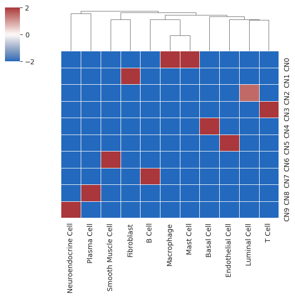
- 热图代表细胞类型在不同细胞 niche 的富集程度
- 横轴代表细胞类型；纵轴代表聚类的细胞 niche；中间的颜色代表富集程度

a

output

AnnData object with n_obs × n_vars = 20820 × 34506
obs: 'imagecol', 'imagerow', 'celltype', 'n_genes_by_counts', 'total_counts', 'CNs_10'
var: 'n_cells_by_counts', 'mean_counts', 'pct_dropout_by_counts', 'total_counts'
uns: 'spatial', 'log1p'
obsm: 'spatial'
layers: 'counts'

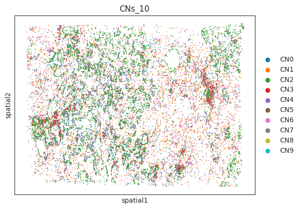
• 细胞 niche 在空间的可视化

sc.pl.embedding(a,"spatial",color=["CNs_10"])

output

/PROJ2/FLOAT/jinwen/apps/miniconda3/envs/COMMOT/lib/python3.10/site-packages/scanpy/plotting/_tools/scatterplots.py:1235: FutureWarning: The default value of 'ignore' for the \`na_action\` parameter in pandas.Categorical.map is deprecated and will be changed to 'None' in a future version. Please set na_action to the desired value to avoid seeing this warning
color_vector = pd.Categorical(values.map(color_map))