ATAC + RNA multi-omics AtaCNV CNV detection and visualization
Document Overview
AtaCNV is a copy number variation (CNV) detection tool specifically developed for single-cell ATAC-seq (scATAC-seq) data. By processing single-cell chromatin accessibility sequencing data, AtaCNV can reveal genetic heterogeneity within complex tissues such as tumor cells at high resolution. It is applicable to the scATAC-seq channel in multi-omics single-cell data, enabling automatic inference and visualization of cell copy number states in complex samples such as tumors.
Significance of CNV Analysis
What is CNV
Copy Number Variation (CNV) refers to structural variations in the quantity of large DNA fragments in the genome, primarily manifested as amplification (gain) or deletion (loss) of chromosomal regions. Under normal conditions, human cells are diploid (each autosome typically has 2 copies); when amplification occurs, the copy number exceeds 2, and when deletion occurs, the copy number is below 2.
CNV is an important driver of the occurrence and progression of various diseases such as cancer. Traditional CNV analysis is primarily based on whole-genome sequencing (WGS) or whole-exome sequencing (WES), which can only provide population-average information. Single-cell CNV analysis infers the copy number state of each cell at single-cell resolution, enabling the revelation of genomic differences and heterogeneity among different cells within tissues.
Two Directions of Single-cell Multi-omics CNV Analysis
Single-cell multi-omics data for CNV analysis mainly has two directions:
- Direction 1: Based on scRNA-seq data - Uses gene expression information to infer CNV, with infercnv as the main tool
- Direction 2: Based on scATAC-seq data - Uses read count information to infer CNV, with main tools including epiAneuFinder, AtaCNV, and CopyscAT
TIP
Introduction to Mainstream Single-cell ATAC-seq CNV Analysis Tools
Currently, commonly used tools for CNV detection in scATAC-seq data include: epiAneuFinder, CopyscAT, and AtaCNV. This guide focuses on the detailed usage of AtaCNV. For other tools, please refer to the technical support documentation for epiAneuFinder and CopyscAT for more information.
Applicable Scenarios and Main Objectives
Suitable sample types:
- Tumor tissue samples (strongly recommended) - Contain numerous CNV events, can reveal tumor heterogeneity and subclonal structure
- Precancerous lesions or developmental abnormality samples - Can detect early genomic structural variations
Unsuitable sample types:
- Normal healthy tissues - Most cells are diploid, lack significant CNV events, CNV analysis has limited significance
Main objectives of single-cell CNV analysis:
- Malignant cell identification - Distinguish malignant cells from non-malignant cells (malignant cells typically exhibit large-scale, non-random CNV patterns)
- Tumor heterogeneity resolution - Identify subclonal populations with different CNV characteristics
- Clonal evolution tracking - Infer tumor clonal evolution relationships through CNV pattern similarity
Implementation of AtaCNV Analysis
Principles of AtaCNV Tool
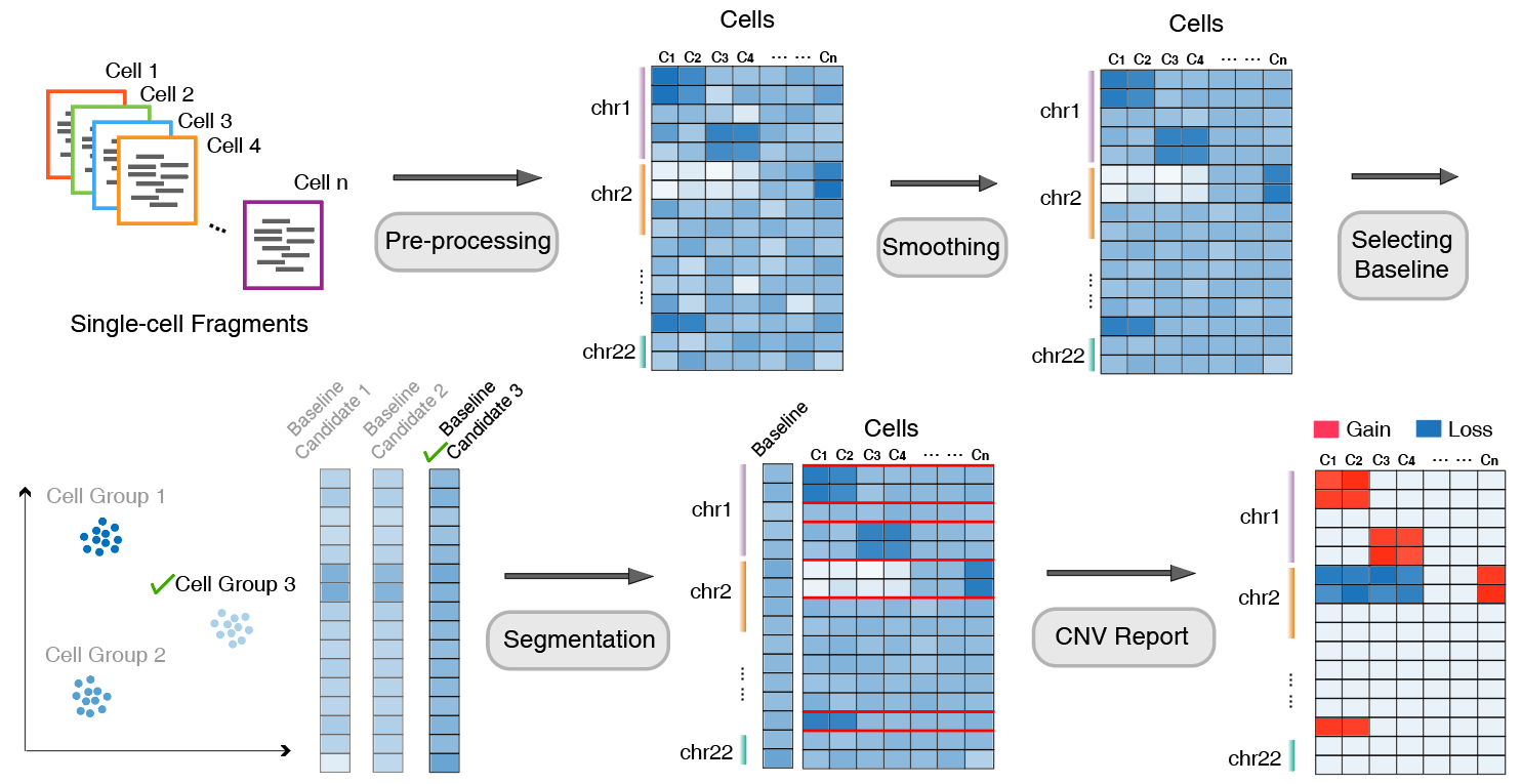
The AtaCNV analysis workflow can be summarized into the following main steps:
Input and preliminary filtering: Takes single-cell Read Count matrices of megabase-pair (1 Mbp) Genomic Fragments as input, first filters cells and Genomic Fragments based on Fragment mappability and zero count numbers.
Data smoothing and bias removal: To reduce extreme noise, AtaCNV smooths the count matrix by fitting a first-order dynamic linear model for each cell. Simultaneously performs cell-based local regression to eliminate potential biases caused by GC content.
Normalization processing:
- If normal cells exist: Normalizes the smoothed count data by comparing with normal cell data, thereby deconvolving copy number signals from confounding factors such as chromatin accessibility.
- If normal cells are lacking: Since tumor single-cell data often contains a large number of non-tumor cells, AtaCNV first clusters cells to identify high-confidence normal cell groups and uses their smoothed depth data as a baseline for normalization.
Joint segmentation and copy number inference: AtaCNV applies a multi-sample BIC-seq algorithm to jointly segment all single cells and estimates the copy number ratio of fragments obtained for each cell.
CNV group discrimination and further inference: Uses copy number ratio data to calculate CNV burden scores for each cell group, and accordingly classifies groups with high CNV burden as malignant cells. For tumor cells, AtaCNV further infers their discrete copy number states through Bayesian methods.
The following figure illustrates the main AtaCNV analysis workflow:
Implementation of AtaCNV Analysis
This approach can precisely quantify the copy number state of each cell across the entire genome, which is a key step in identifying malignant cells and resolving tumor heterogeneity. When implementing actual projects, it is recommended to select appropriate normalization modes based on data characteristics to obtain the most accurate CNV detection results.
# Load AtaCNV package and prepare data
library("AtaCNV")

# Generate count matrix from fragment file and cell barcodes (or directly read preprocessed data)
fragment_file <- "your_fragment_file.tsv.gz"
cell_barcodes <- read.csv("your_cell_barcodes.tsv", header=FALSE)
count <- generate_input(
  fragment_file = fragment_file,
  cell_barcodes = cell_barcodes,
  genome = "hg19",  # or "hg38", "mm10"
  output_dir = "./"
)

# Read example data
#cell_info <- readRDS("./example/cell_info.rds")
#count_paired <- readRDS("./example/count_paired.rds")  # Matched normal sample

# Normalization: Select mode based on available information
# Mode 1: Matched normal sample (most reliable)
norm_re1 <- AtaCNV::normalize(
  count,
  genome = "hg19",
  mode = "matched normal sample",
  cell_cluster = cell_info$cluster,
  count_paired = count_paired,
  output_dir = "./",
  output_name = "norm_re1.rds"
)

# Mode 2: Known normal cells
# norm_re2 <- AtaCNV::normalize(
#   count
#   genome = "hg19"
#   mode = "normal cells"
#   normal_cells = (cell_info$cell_type == "normal")
#   output_dir = "./"
#   output_name = "norm_re2.rds"
# )

# Mode 3: All cells (only applicable when tumor purity is low)
# norm_re3 <- AtaCNV::normalize(
#   count
#   genome = "hg19"
#   mode = "all cells"
#   cell_cluster = cell_info$cluster
#   output_dir = "./"
#   output_name = "norm_re3.rds"
# )

# Mode 4: Automatic identification (when no additional information is available)
# norm_re4 <- AtaCNV::normalize(
#   count
#   genome = "hg19"
#   mode = "none"
#   cell_cluster = cell_info$cluster
#   output_dir = "./"
#   output_name = "norm_re4.rds"
# )

# Segmentation: Use BIC-seq algorithm to infer CNA breakpoints and estimate copy number ratios
seg_re <- calculate_CNV(
  norm_count = norm_re1$norm_count,
  baseline = norm_re1$baseline,
  output_dir = "./",
  output_name = "seg_re.rds"
)

# Optional: Infer copy number state
CN_state <- estimate_cnv_state_cluster(
  count = count,
  genome = "hg19",
  copy_ratio = norm_re1$copy_ratio,
  bkp = seg_re$bkp,
  label = cell_info$cell_type
)

# Heatmap visualization
plot_heatmap(
  copy_ratio = seg_re$copy_ratio,
  cell_cluster = cell_info$cluster,
  output_dir = "./",
  output_name = "copy_ratio.png"
)
TIP
Normalization Mode Selection
AtaCNV provides four normalization modes to estimate baseline read counts for non-tumor cells:
- Mode 1 (matched normal sample): Most reliable, prioritize when matched non-tumor samples are available
- Mode 2 (normal cells): Use when normal cells in the sample are known, can preliminarily identify normal cells by estimating marker gene expression from scATAC-seq data using tools such as ArchR
- Mode 3 (all cells): Only applicable when tumor purity is low
- Mode 4 (none): Use when no additional information is available, AtaCNV will automatically identify the most likely normal cells, but accuracy may be lower
If no pre-existing clustering results are available, the cell_cluster parameter can be omitted, and AtaCNV will automatically perform clustering based on the count matrix.
CNV Results Display--Copy Number Variation Heatmap
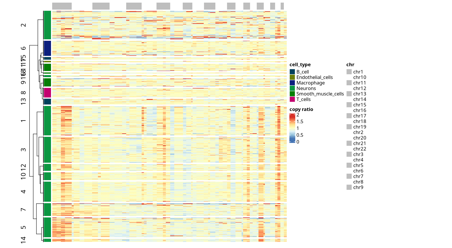
The copy number variation heatmap is the core visualization result of CNV analysis, comprehensively displaying the copy number state of all cells across the entire genome:
In the copy number variation heatmap, each row represents a cell, and each column represents a continuous interval (bin) on the genome. All columns are arranged in order of chromosomal physical positions, sequentially from chromosome 1 to sex chromosomes (if present). The color of each column reflects the relative copy number value of that interval in the corresponding cell: for example, red indicates copy number amplification (gain), and blue indicates copy number deletion (loss). The heatmap shows that the number of columns between adjacent chromosomes may differ significantly (e.g., some have 3 columns, some have 4 columns, some have only 1 column), reflecting subtle differences in chromosome length.
Frequently Asked Questions
Q1: How to select an appropriate normalization mode?
A: AtaCNV provides four normalization modes, with selection recommendations as follows:
- Mode 1 (matched normal sample): Most reliable, prioritize when matched non-tumor samples are available
- Mode 2 (normal cells): Use when normal cells in the sample are known, can preliminarily identify normal cells by estimating marker gene expression from scATAC-seq data using tools such as ArchR
- Mode 3 (all cells): Only applicable when tumor purity is low, uses all cells to construct baseline
- Mode 4 (none): Use when no additional information is available, AtaCNV will automatically identify the most likely normal cells, but accuracy may be lower
- Recommendation: If possible, try to use Mode 1 or Mode 2 to obtain more accurate CNV detection results
Q2: How to interpret the values in copy number state results?
A: In copy number state inference results:
- 0.5: Indicates copy number deletion (loss), the copy number of this region in the corresponding cell is below normal levels
- 1: Indicates copy number neutral (neutral), i.e., normal diploid state
- 1.5: Indicates copy number amplification (gain), the copy number of this region in the corresponding cell is above normal levels
- These values reflect the copy number state of each cell in each genomic interval (bin) and can be used to identify malignant cells and subclonal structure
References
[1] WANG X, et al. Detecting copy-number alterations from single-cell chromatin sequencing data by AtaCNV[J]. Cell Reports Methods, 2025, 5(1).