ATAC + RNA multi-omics CopyscAT CNV inference and tumor cell identification
Document Overview
CopyscAT can infer copy number variation (CNV) based on scATAC-seq data to assist in identifying cancer cells. It helps study the relationship between chromosomal changes and epigenomic states of different subclones within complex tumors (such as glioblastoma), and analyze how genetic variations affect cellular molecular phenotypes. CopyscAT is particularly suitable for exploring the interaction between genetics and epigenetics in highly heterogeneous tumors, as well as the mechanisms of interaction between tumor cells and the microenvironment.
Single-cell multi-omics data contains scATAC-seq information, and CopyscAT can be used to perform CNV analysis on scATAC-seq in multi-omics data to reveal tumor cell heterogeneity.
Significance of CNV Analysis
What is CNV
Copy Number Variation (CNV) refers to structural variations in the quantity of large DNA fragments in the genome, primarily manifested as amplification (gain) or deletion (loss) of chromosomal regions. Under normal conditions, human cells are diploid (each autosome typically has 2 copies); when amplification occurs, the copy number exceeds 2, and when deletion occurs, the copy number is below 2.
CNV is an important driver of the occurrence and progression of various diseases such as cancer. Traditional CNV analysis is primarily based on whole-genome sequencing (WGS) or whole-exome sequencing (WES), which can only provide population-average information. Single-cell CNV analysis infers the copy number state of each cell at single-cell resolution, enabling the revelation of genomic differences and heterogeneity among different cells within tissues.
Two Directions of Single-cell Multi-omics CNV Analysis
Single-cell multi-omics data for CNV analysis mainly has two directions:
- Direction 1: Based on scRNA-seq data - Uses gene expression information to infer CNV, with InferCNV as the main tool
- Direction 2: Based on scATAC-seq data - Uses Read count information to infer CNV, with main tools including epiAneuFinder, AtaCNV, and CopyscAT
TIP
Introduction to Mainstream Single-cell ATAC-seq CNV Analysis Tools
Currently, commonly used tools for CNV detection in scATAC-seq data include: epiAneuFinder, CopyscAT, and AtaCNV. This guide focuses on the detailed usage of CopyscAT. For other tools, please refer to the relevant documentation for AtaCNV and epiAneuFinder for more information.
Applicable Scenarios and Main Objectives
Suitable sample types:
- Tumor tissue samples (strongly recommended) - Contain numerous CNV events, can reveal tumor heterogeneity and subclonal structure
- Precancerous lesions or developmental abnormality samples - Can detect early genomic structural variations
Unsuitable sample types:
- Normal healthy tissues - Most cells are diploid, lack significant CNV events, CNV analysis has limited significance
Main objectives of single-cell CNV analysis:
- Malignant cell identification - Distinguish malignant cells from non-malignant cells (malignant cells typically exhibit large-scale, non-random CNV patterns)
- Tumor heterogeneity resolution - Identify subclonal populations with different CNV characteristics
- Clonal evolution tracking - Infer tumor clonal evolution relationships through CNV pattern similarity
Implementation of CopyscAT Analysis
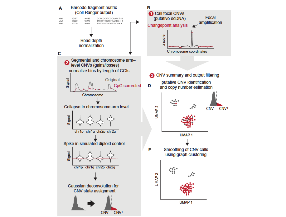
Principles of CopyscAT Tool
CopyscAT uses single-cell epigenomic data to infer copy number variation (CNV), thereby defining and identifying cancer cells. The core principle of this tool is to use the number of Reads mapped to Genomic regions in scATAC-seq data as a proxy indicator of DNA copy number in that region.
The CopyscAT analysis workflow includes the following key steps:
- Data input: Accepts Barcode-Fragment matrices generated by seekARC as input
- Data normalization: Performs normalization processing on coverage matrices to generate normalized matrices
- CNV detection:
- Local CNV detection: Infers local CNV (such as ecDNA, i.e., extrachromosomal DNA) through large Peaks in normalized coverage matrices
- Fragment and Chromosome arm level CNV detection: Uses normalized matrices to infer CNV at Fragment level and Chromosome arm level
- Double minutes detection: Identifies High copy number amplification regions in the genome
- Cell assignment: Uses consensus clustering methods to finally determine cell grouping and CNV states
A key advantage of CopyscAT is its ability to automatically identify non-tumor cells and use them as controls, thereby more accurately detecting CNV in tumor cells. This tool is particularly suitable for processing complex samples with high levels of intratumoral heterogeneity.
The following figure illustrates the main CopyscAT analysis workflow:
Implementation of CopyscAT Analysis
The CopyscAT analysis workflow includes initialization setup, data normalization, CNV detection, and result output steps. The following is a complete usage example:
Initial One-time Setup
library("devtools")

# STEP 1: Replace "~/CopyscAT" with your git clone repository path
install("~/CopyscAT")

# Or install from GitHub (some R versions may error due to code warnings, use the following line to resolve)
Sys.setenv("R_REMOTES_NO_ERRORS_FROM_WARNINGS" = "true")
install_github("spcdot/copyscat")

# Load package
library(CopyscAT)

# Load the genome you are using
library(BSgenome.Hsapiens.UCSC.hg38)

# Generate reference files - This will create genome chrom.sizes file, cytobands file, and CpG file
generateReferences(BSgenome.Hsapiens.UCSC.hg38,
                   genomeText = "hg38",
                   tileWidth = 1e6,
                   outputDir = "~")
Regular Workflow
# Initialize environment (Note: This step needs to be executed for each CopyscAT session)
initialiseEnvironment(genomeFile="~/hg38_chrom_sizes.tsv",
                      cytobandFile="~/hg38_1e+06_cytoband_densities_granges.tsv",
                      cpgFile="~/hg38_1e+06_cpg_densities.tsv",
                      binSize=1e6,
                      minFrags=1e4,
                      cellSuffix=c("-1","-2"),
                      lowerTrim=0.5,
                      upperTrim=0.8)

# Set default output directory and filename
setOutputFile("~","samp_dataset")

# ===== PART 1: Initial Data Normalization =====

# Read input data (if using your own file, replace with the following code)
# scData <- readInputTable("myInputFile.tsv")
scData <- scDataSamp  # Use package example data

# Normalize matrix
scData_k_norm <- normalizeMatrixN(scData,
                                   logNorm = FALSE,
                                   maxZero=2000,
                                   imputeZeros = FALSE,
                                   blacklistProp = 0.8,
                                   blacklistCutoff=125,
                                   dividingFactor=1,
                                   upperFilterQuantile = 0.95)

# Collapse to chromosome arm level
summaryFunction <- cutAverage
scData_collapse <- collapseChrom3N(scData_k_norm,
                                    summaryFunction=summaryFunction,
                                    binExpand = 1,
                                    minimumChromValue = 100,
                                    logTrans = FALSE,
                                    tssEnrich = 1,
                                    logBase=2,
                                    minCPG=300,
                                    powVal=0.73)

# Apply additional filtering
scData_collapse <- filterCells(scData_collapse,
                                minimumSegments = 40,
                                minDensity = 0.1)

# Display unscaled chromosome list
graphCNVDistribution(scData_collapse, outputSuffix = "test_violinsn2")

# Compute centers
median_iqr <- computeCenters(scData_collapse,
                              summaryFunction=summaryFunction)

# ===== PART 2: Chromosome Level CNV Assessment =====

# OPTION 1: Use all cells to generate "normal" control to identify chromosome level amplification
candidate_cnvs <- identifyCNVClusters(scData_collapse,
                                       median_iqr,
                                       useDummyCells = TRUE,
                                       propDummy=0.25,
                                       minMix=0.01,
                                       deltaMean = 0.03,
                                       deltaBIC2 = 0.25,
                                       bicMinimum = 0.1,
                                       subsetSize=600,
                                       fakeCellSD = 0.08,
                                       uncertaintyCutoff = 0.55,
                                       summaryFunction=summaryFunction,
                                       maxClust = 4,
                                       mergeCutoff = 3,
                                       IQRCutoff= 0.2,
                                       medianQuantileCutoff = 0.4)

# Cleanup step
candidate_cnvs_clean <- clusterCNV(initialResultList = candidate_cnvs,
                                    medianIQR = candidate_cnvs[[3]],
                                    minDiff=1.5)

# Final results and annotation
final_cnv_list <- annotateCNV4(candidate_cnvs_clean,
                                saveOutput=TRUE,
                                outputSuffix = "clean_cnv",
                                sdCNV = 0.5,
                                filterResults=TRUE,
                                filterRange=0.8)

# OPTION 2: Automatically identify non-tumor cells and use them as controls
# Note: This method is still experimental, use when copy number calls from Option A are unreasonable (e.g., baseline seems incorrect)
# Works best when tumor cell purity <90% (very small non-tumor cell populations may be missed)

# Running this step requires after filterCells
nmf_results <- identifyNonNeoplastic(scData_collapse,
                                     methodHclust="ward.D",
                                     cutHeight = 0.4)

# Save non-tumor cell identification results
write.table(x=rownames_to_column(data.frame(nmf_results$cellAssigns),
                                  var="Barcode"),
            file=str_c(scCNVCaller$locPrefix,
                       scCNVCaller$outPrefix,
                       "_nmf_clusters.csv"),
            quote=FALSE,
            row.names = FALSE,
            sep=",")

print(paste("Normal cluster is: ",nmf_results$clusterNormal))

# Alternative CNV calling method using normal cells as background
# Compute center trend based only on normal cells
median_iqr <- computeCenters(scData_collapse %>%
                                select(chrom,nmf_results$normalBarcodes),
                              summaryFunction=summaryFunction)

# CNV calling using normal cells
candidate_cnvs <- identifyCNVClusters(scData_collapse,
                                       median_iqr,
                                       useDummyCells = TRUE,
                                       propDummy=0.25,
                                       minMix=0.01,
                                       deltaMean = 0.03,
                                       deltaBIC2 = 0.25,
                                       bicMinimum = 0.1,
                                       subsetSize=800,
                                       fakeCellSD = 0.09,
                                       uncertaintyCutoff = 0.65,
                                       summaryFunction=summaryFunction,
                                       maxClust = 4,
                                       mergeCutoff = 3,
                                       IQRCutoff = 0.25,
                                       medianQuantileCutoff = -1,
                                       normalCells=nmf_results$normalBarcodes)

candidate_cnvs_clean <- clusterCNV(initialResultList = candidate_cnvs,
                                    medianIQR = candidate_cnvs[[3]],
                                    minDiff=1.0)

final_cnv_list <- annotateCNV4(candidate_cnvs_clean,
                                saveOutput=TRUE,
                                outputSuffix = "clean_cnv",
                                sdCNV = 0.6,
                                filterResults=TRUE,
                                filterRange=0.4)

# Or use annotateCNV4B and input normalBarcodes
final_cnv_list <- annotateCNV4B(candidate_cnvs_clean,
                                 nmf_results$normalBarcodes,
                                 saveOutput=TRUE,
                                 outputSuffix = "clean_cnv_b2",
                                 sdCNV = 0.6,
                                 filterResults=TRUE,
                                 filterRange=0.4,
                                 minAlteredCellProp = 0.5)

# ===== PART 2B: Smooth CNV Calls Using Clustering =====
smoothedCNVList <- smoothClusters(scDataSampClusters,
                                   inputCNVList = final_cnv_list[[3]],
                                   percentPositive = 0.4,
                                   removeEmpty = FALSE)

# ===== PART 3: Identify Double Minutes/Amplification =====
# Note: This step is slow and may take about 5 minutes
library(compiler)
dmRead <- cmpfun(identifyDoubleMinutes)

# minThreshold is a time-saving option that won't call breakpoints on any cell with max Z score less than 4
dm_candidates <- dmRead(scData_k_norm,
                        minCells=100,
                        qualityCutoff2 = 100,
                        minThreshold = 4)

write.table(x=dm_candidates,
            file=str_c(scCNVCaller$locPrefix,
                       scCNVCaller$outPrefix,
                       "samp_dm.csv"),
            quote=FALSE,
            row.names = FALSE,
            sep=",")

# ===== PART 4: Call Fragment Deletion/Amplification (only on datasets with NMF-detected normal cells) =====
altered_segments <- getAlteredSegments(scData_k_norm,
                                       nmf_results,
                                       lossThreshold = 0.6)

write.table(x=altered_segments,
            file=str_c(scCNVCaller$locPrefix,
                       scCNVCaller$outPrefix,
                       "samp_segments.csv"),
            quote=FALSE,
            row.names = FALSE,
            sep=",")

# ===== PART 5: Quantify Cycling Cells =====
# Use signal from specific chromosome (we use X chromosome as it is usually not altered in our samples)
# If X chromosome has known alterations in your sample, try using a different chromosome
barcodeCycling <- estimateCellCycleFraction(scData,
                                            sampName="sample",
                                            cutoff=1000)

write.table(barcodeCycling[order(names(barcodeCycling))]==max(barcodeCycling),
            file=str_c(scCNVCaller$locPrefix,
                       scCNVCaller$outPrefix,
                       "_cycling_cells.tsv"),
            sep="\t",
            quote=FALSE,
            row.names=TRUE,
            col.names=FALSE)
TIP
Key Points of CopyscAT Analysis
CopyscAT provides two CNV detection strategies:
- Option 1 (Recommended): Use all cells to generate controls, suitable for most cases
- Option 2: Automatically identify non-tumor cells as controls, suitable for samples with low tumor purity (<90%)
Key Parameter Descriptions:
- binSize: Genomic window size, default 1Mb
- minFrags: Minimum fragments per cell, default 10000
- blacklistProp: Blacklist region filtering proportion, default 0.8
- cutHeight: Cutting height during NMF clustering, needs to be adjusted based on actual data
It is recommended to run with default parameters first, then make appropriate adjustments based on result quality.
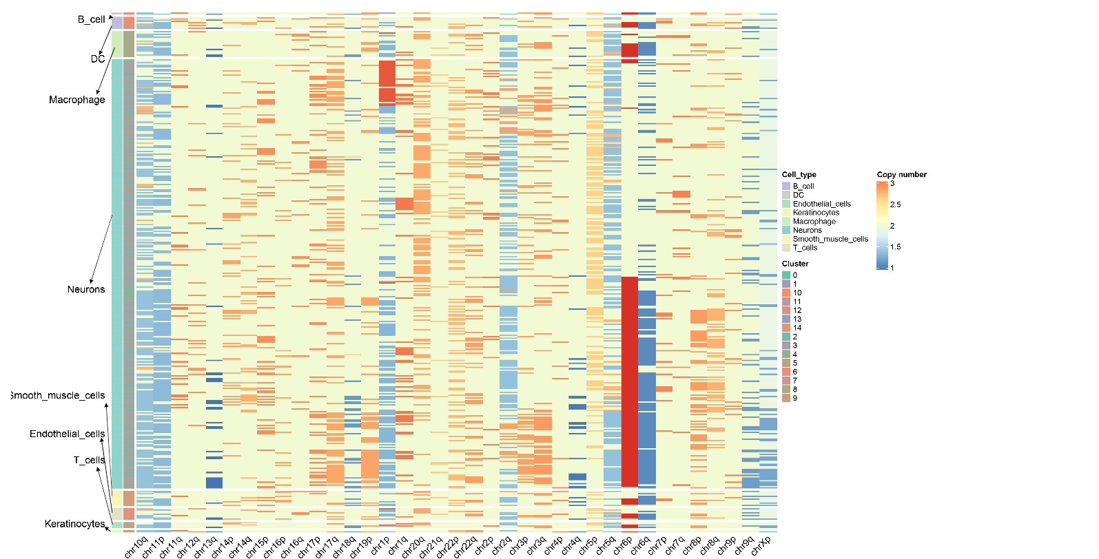
CNV Results Display--Copy Number Variation Heatmap
The copy number variation heatmap is the core visualization result of CNV analysis, comprehensively displaying the copy number state of all cells across the entire genome:
Meaning of rows and columns:
- Each row represents a Cell
- Each column represents a Chromosome arm, and the color of the heatmap represents CNV scores
- The order of columns corresponds to the linear arrangement of the genome from Chromosome 1 to Sex chromosomes (if retained)
Color mapping:
- Copy number values around 2 indicate normal diploid state
- Copy number between 1~2 indicates chromatin deletion, closer to 1 indicates more severe deletion
- Copy number between 2~3 indicates chromatin amplification, closer to 3 indicates more severe amplification
- Redder colors indicate more severe amplification, bluer colors indicate more severe deletion
Cell annotation:
- The color bars on the left side of the heatmap represent arranging cells according to cell type and cell clustering
- CopyscAT uses consensus clustering methods to finally determine cell CNV states and grouping
- Malignant cells typically exhibit obvious CNV patterns (large-scale amplification or deletion), while non-malignant cells (such as T cells, B cells) maintain relatively normal diploid state
Frequently Asked Questions
Q1: How to select an appropriate CNV detection strategy?
A: CopyscAT provides two CNV detection strategies:
- Option 1: Use all cells to generate controls. Suitable for most cases, especially when tumor cells account for a high proportion in the sample
- Option 2: Automatically identify non-tumor cells as controls. Suitable for samples with low tumor purity (<90%), can set baseline more accurately. However, it should be noted that if the non-tumor cell population is very small, it may be missed
Q2: How to interpret the values in copy number results?
A: In copy number inference results:
- Close to 2: Indicates normal copy number (diploid state), meaning the region maintains normal copy number in the corresponding cell
- Between 1~2: Indicates copy number deletion (loss), the copy number of this region in the corresponding cell is below normal levels, closer to 1 indicates more severe deletion
- Between 2~3: Indicates copy number amplification (gain), the copy number of this region in the corresponding cell is above normal levels, closer to 3 indicates more severe amplification
- These values reflect the copy number state of each cell in each genomic window and can be used to identify malignant cells and subclonal structure
Q3: How to adjust NMF clustering parameters?
A: When using the identifyNonNeoplastic function, if results are not ideal, the following parameters can be adjusted:
- cutHeight: Height for cutting dendrogram, default 0.6. If clustering separation is poor, this value can be reduced (e.g., 0.4)
- nmfComponents: Number of NMF components, default 5. Can be adjusted based on sample complexity
- estimatedCellularity: Estimated tumor cell proportion, default 0.8. If the tumor purity of the sample is known, this parameter can be adjusted
Q4: What are the advantages of CopyscAT compared to other CNV detection tools?
A: The main advantages of CopyscAT include:
- Automatic identification of normal cells: Can automatically identify non-tumor cells in samples and use them as controls, improving CNV detection accuracy
- Multi-level CNV detection: Can detect local CNV (such as ecDNA), fragment level CNV, and chromosome arm level CNV
- Double minutes detection: Can identify high copy number amplification regions (double minutes) in the genome
- Cell cycle analysis: Provides cell cycle fraction estimation function, helpful for understanding cell states
- Suitable for complex tumors: Particularly suitable for processing complex samples with high levels of intratumoral heterogeneity, such as glioblastoma
Q5: How to handle large sample data?
A: For very large datasets:
- Data can be subset sampled (e.g., using
subsetSizeparameter) - Analysis can be run separately on different cell populations, then merge results
- For time-consuming steps such as double minutes detection, consider running only on specific cell populations
References
[1] NIKOLIC A, SINGHAL D, ELLESTAD K, et al. Copy-scAT: Deconvoluting single-cell chromatin accessibility of genetic subclones in cancer[J]. Science Advances, 2021, 7(42): eabg6045.