Basic Analysis
"Basic Analysis" is the initial module of the analysis workflow. It performs gene and mitochondrial filtering, batch correction, and clustering to retain high-quality cells for downstream analyses. The steps for creating the workflow and running filtering, integration, and clustering are as follows:
Initial Stage
Click Create Process to create a single-cell analysis workflow. Projects typically begin with bulk cluster analysis of selected samples, and you can later choose annotated cell types for subcluster analysis.
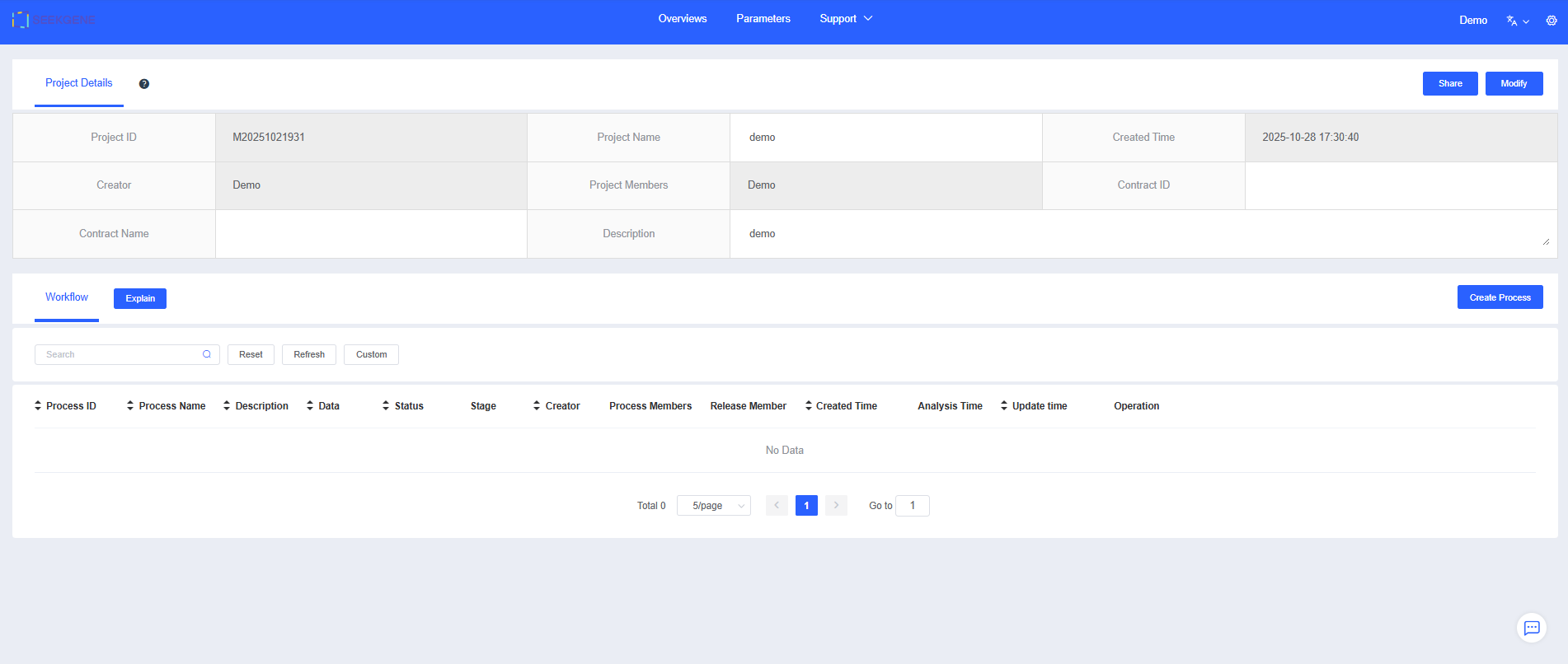
Enter a "Process Name" and "Description" to help you find and understand the workflow later.
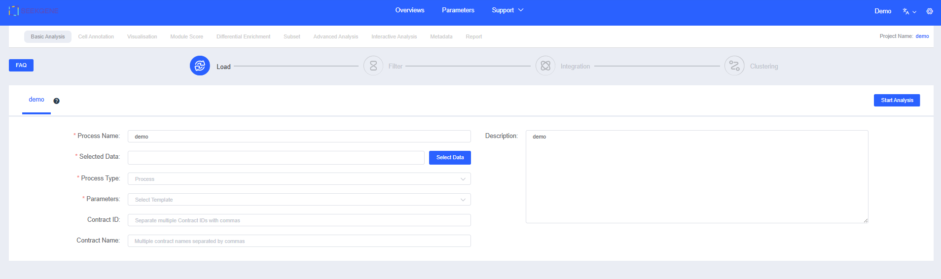
Click Select Data to choose the samples for analysis. You can pick pre-integrated multi-sample data or select multiple individual samples for filtering and integration.
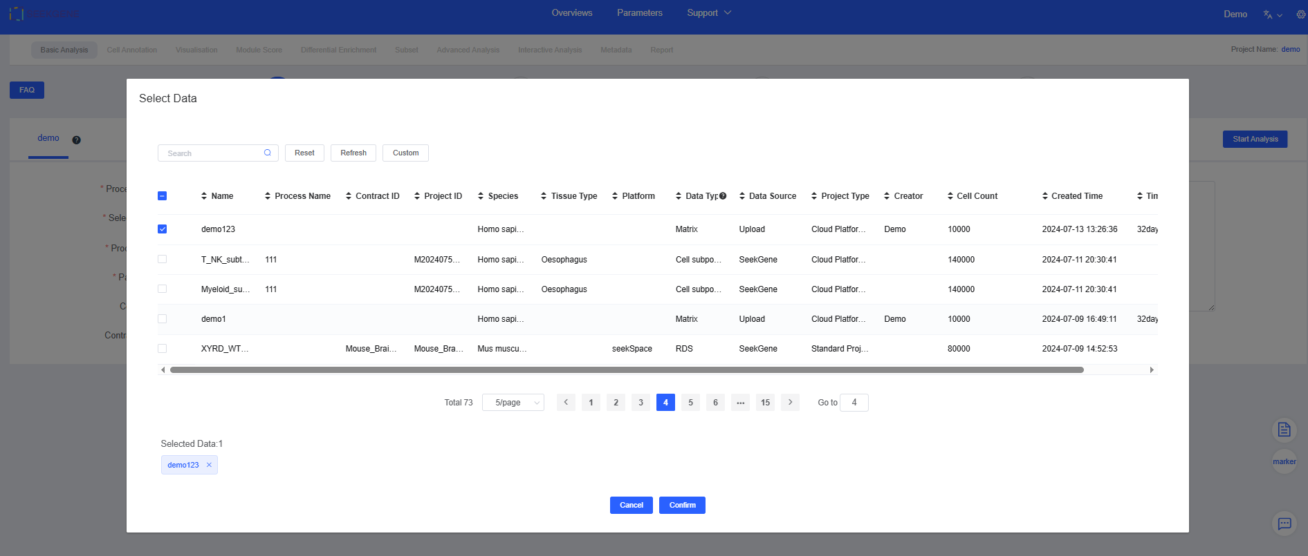
NOTE
See Datas for detailed data sources.
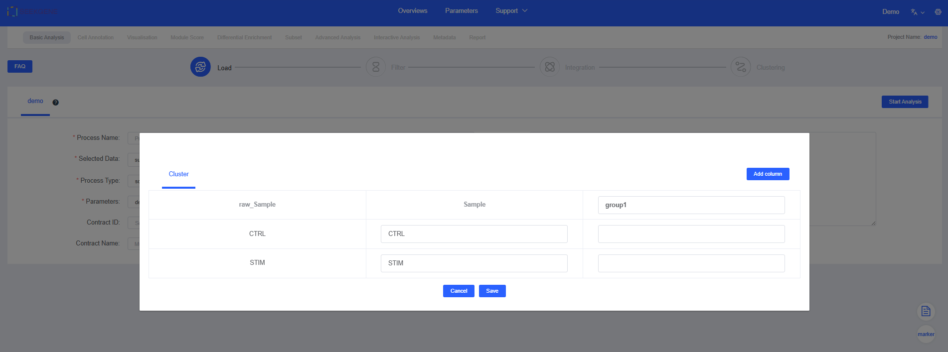
- Click Group to add grouping information (optional). You can also add grouping information in later modules; refer to Plotting Tools for the label feature and Differential Enrichment for grouping functionality.
Filter
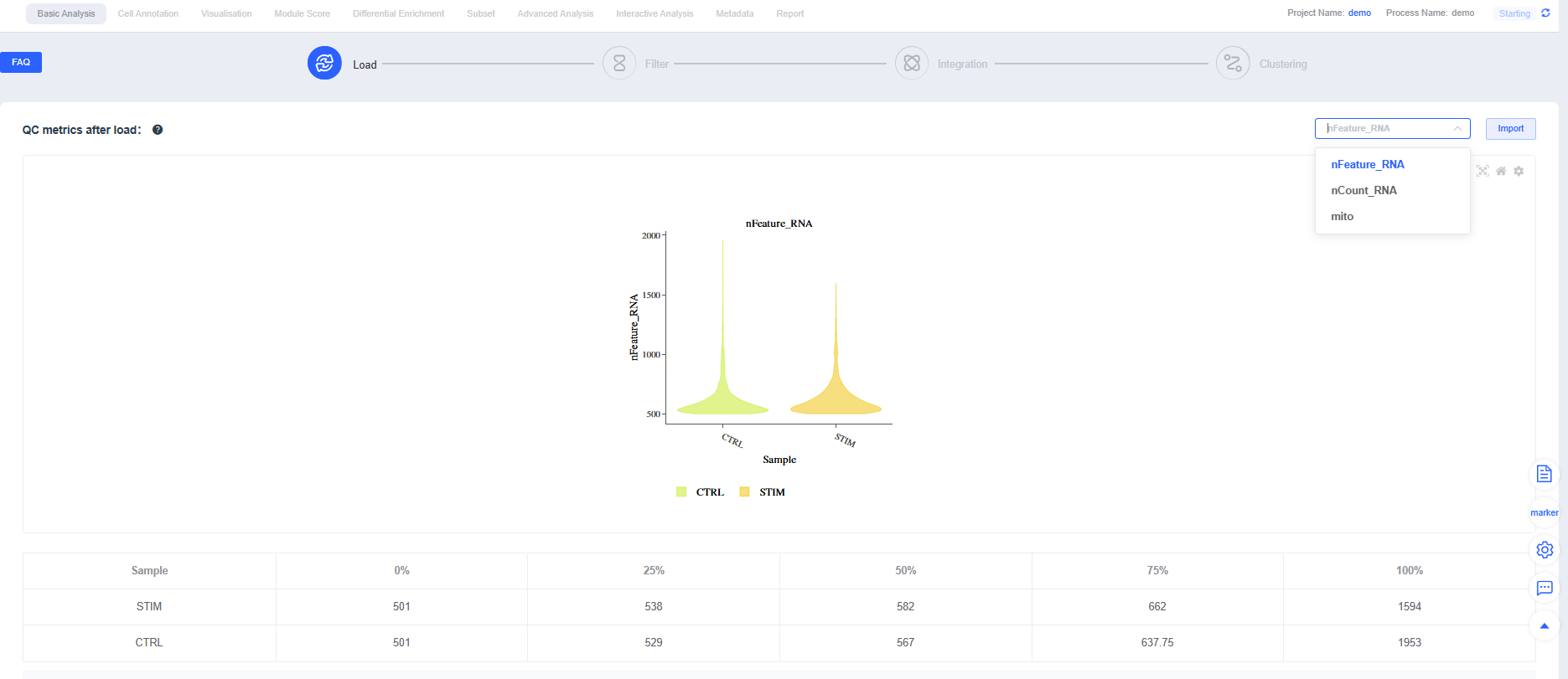
- After you click Start Analysis, the "Charts & Data" section summarizes UMI counts, mitochondrial proportions, and gene expression to provide an overview of sample quality.
NOTE
Metric definitions (scRNA-seq):
- nCount_RNA: Total UMI count per cell, reflecting sequencing depth and transcript abundance
- nFeature_RNA: Number of genes detected per cell, reflecting expression complexity
- Mitochondrial proportion (mito): Percentage of UMIs from mitochondrial genes; elevated levels often indicate apoptosis or damage (increase the allowance slightly for highly metabolic tissues)
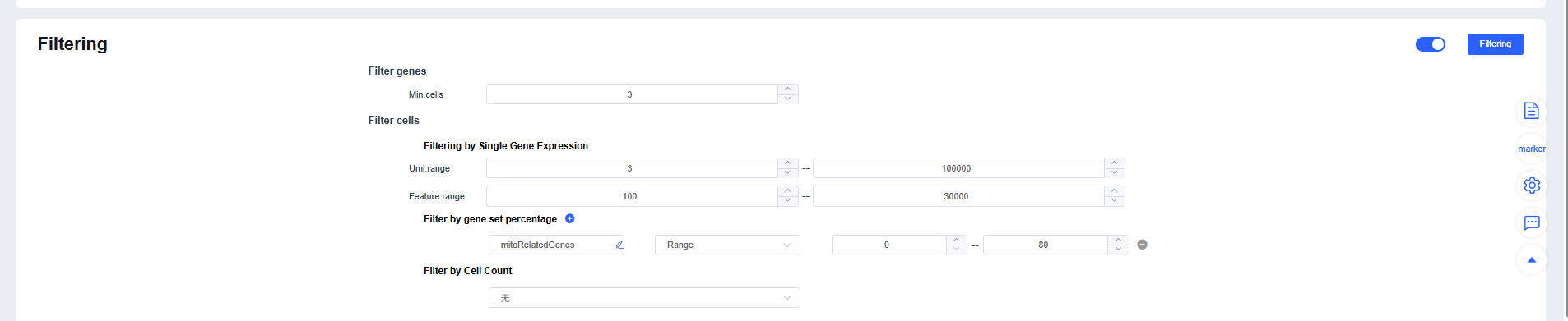
- Expand the panel to view default parameters. You can reference filtering settings reported in published single-cell studies when running Filtering.
TIP
If you selected pre-integrated data, clicking Filtering prompts you to decide whether to skip the filtering and integration steps. Skip them when no parameter adjustments are needed; cancel the skip to rerun filtering and integration when thresholds must be tuned.
IMPORTANT
Filtering strategy recommendations:
- Use MAD-based dynamic thresholds for mt% or reference an upper limit of 10%-20%.
- Identify extreme outliers in nCount_RNA/nFeature_RNA using quantiles or the upper whisker of a boxplot.
- For multi-sample datasets, perform balanced subsampling by cell count to prevent sample size from dominating clustering.
- Relax thresholds for highly metabolic tissues (heart/kidney/liver) or samples rich in immune/granulocyte populations to avoid removing genuine cells.
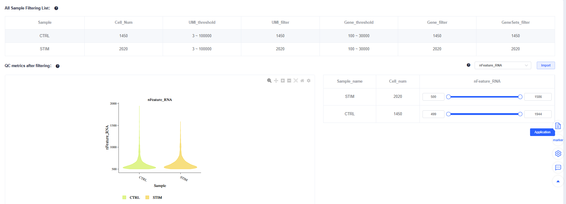
After Filtering, review the post-filtering quality metrics for each sample. You can fine-tune individual samples to maintain consistent overall quality.
CAUTION
Avoid mechanically "raising cell counts" (for example, loosening lower bounds purely by intuition). If the waterfall plot lacks a clear inflection point, background is high, or low-UMI populations are abnormal, forcing recovery reduces downstream stability. Doublet detection guidelines:
- Flag high-end tails in nCount_RNA/nFeature_RNA distributions (extreme values on the right).
- Check for mutually exclusive markers co-expressed or "bridge" cells between two UMAP clusters.
- In tumor projects, combine CNV evidence.
- Filter cautiously: remove cells only when multiple lines of evidence agree, and rerun integration and clustering afterward to confirm consistency.
Integration
Once QC passes, click Integration. Four integration methods are available; CCA, Harmony, and RPCA perform batch correction across multiple samples.
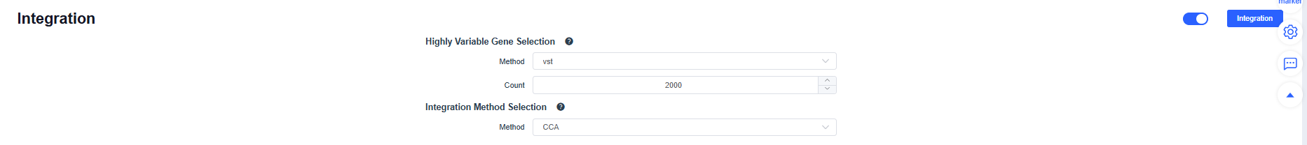
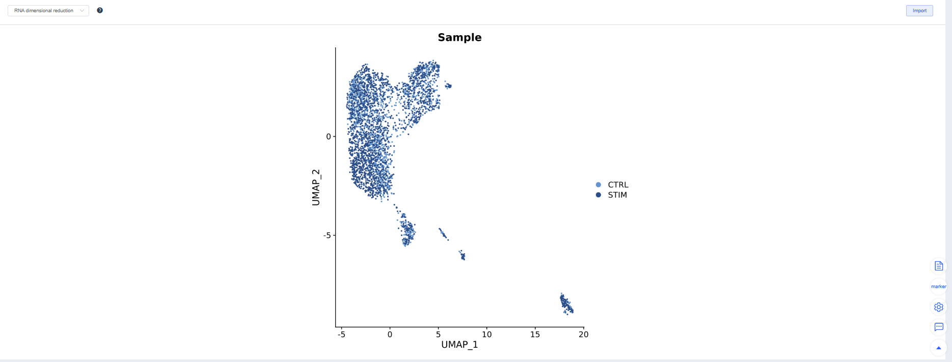
After Integration, the system displays the integration results. Adjust parameters and rerun integration as needed. Try multiple methods and choose the one that best suits subsequent analyses.
TIP
Choosing an integration method:
- Weak batch effect: merge directly to avoid overcorrection.
- Moderate batch effect: CCA or RPCA.
- Pronounced or heterogeneous batches: Harmony is more robust.
TIP
Three criteria for evaluating integration quality:
- Batch mixing: The same cell type mixes evenly across samples on UMAP/TSNE.
- Biological signal retention: Classic marker gradients and cluster boundaries remain clear, and differential/enrichment results meet expectations.
- Over/under-correction warnings: Overcorrection flattens differences, while under-correction produces clusters grouped by batch.
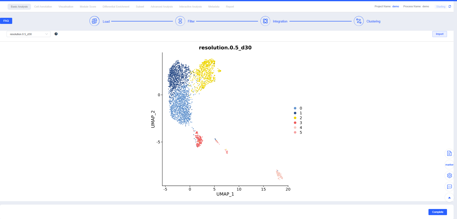
Clustering
After confirming Integration, proceed with Clustering. You can create clustering results at multiple resolutions; higher resolutions yield more clusters. Additional resolutions can be added in later modules.

TIP
Clustering tuning and troubleshooting:
- Elbow method: Use the PCA elbow point as the starting value for dims; increase it as the cell count grows.
- Subset reclustering: Recluster large categories (e.g., T cells) separately to highlight intra-category heterogeneity. If dims are too low, key heterogeneity may be missed; if too high, overclustering and amplified noise can occur. Optimize based on elbow points and reproducibility.
Complete
If no further adjustments are needed after Clustering, click Complete to jump to the Cell Annotation module and begin downstream single-cell analyses. This step takes some time—please be patient.