"Basic Analysis" is the initial module of the analysis workflow. It performs gene and mitochondrial filtering, batch correction, and clustering to retain high-quality cells for downstream analyses. The steps for creating the workflow and running filtering, integration, and clustering are as follows:

Initial Stage

1. Click Create Process to create a single-cell analysis workflow. Projects typically begin with bulk cluster analysis of selected samples, and you can later choose annotated cell types for subcluster analysis.

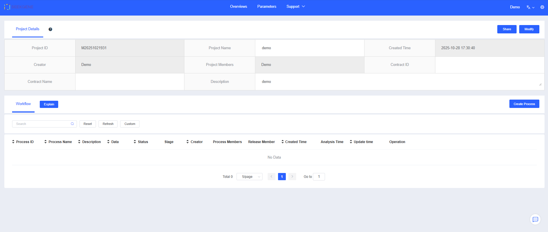
2. Enter a "Process Name" and "Description" to help you find and understand the workflow later.

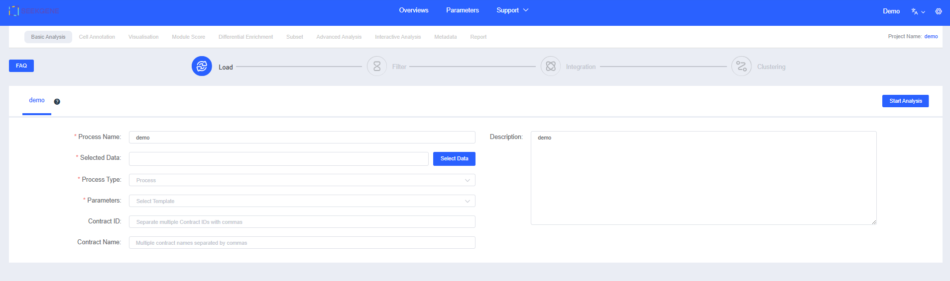
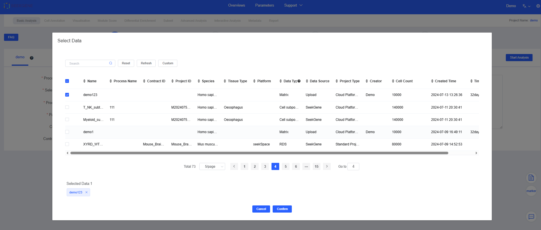
3. Click Select Data to choose the samples for analysis. You can pick pre-integrated multi-sample data or select multiple individual samples for filtering and integration.

NOTE

See Datas for detailed data sources.

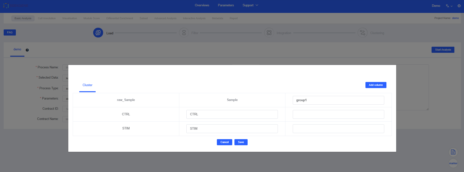
4. Click Group to add grouping information (optional). You can also add grouping information in later modules; refer to Plotting Tools for the label feature and Differential Enrichment for grouping functionality.

Filter

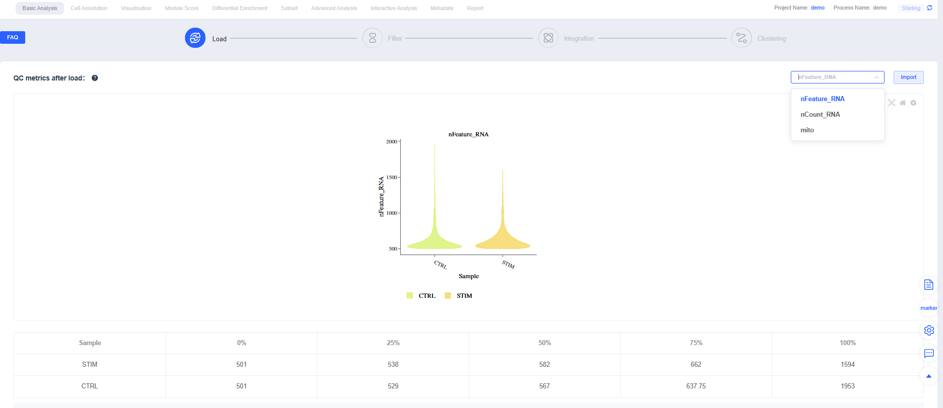
1. After you click Start Analysis, the "Charts & Data" section summarizes UMI counts, mitochondrial proportions, and gene expression to provide an overview of sample quality.

NOTE

Metric definitions (scRNA-seq):

• nCount_RNA: Total UMI count per cell, reflecting sequencing depth and transcript abundance
• nFeature_RNA: Number of genes detected per cell, reflecting expression complexity
• Mitochondrial proportion (mito): Percentage of UMIs from mitochondrial genes; elevated levels often indicate apoptosis or damage (increase the allowance slightly for highly metabolic tissues)

2. Expand the panel to view default parameters. You can reference filtering settings reported in published single-cell studies when running Filtering.

TIP

If you selected pre-integrated data, clicking Filtering prompts you to decide whether to skip the filtering and integration steps. Skip them when no parameter adjustments are needed; cancel the skip to rerun filtering and integration when thresholds must be tuned.

IMPORTANT

Filtering strategy recommendations:

• Use MAD-based dynamic thresholds for mt% or reference an upper limit of 10%-20%.
• Identify extreme outliers in nCount_RNA/nFeature_RNA using quantiles or the upper whisker of a boxplot.
• For multi-sample datasets, perform balanced subsampling by cell count to prevent sample size from dominating clustering.
• Relax thresholds for highly metabolic tissues (heart/kidney/liver) or samples rich in immune/granulocyte populations to avoid removing genuine cells.

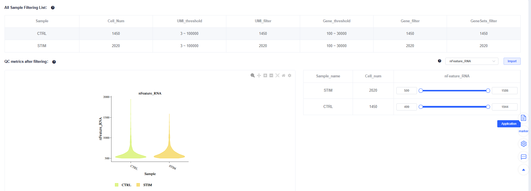
3. After Filtering, review the post-filtering quality metrics for each sample. You can fine-tune individual samples to maintain consistent overall quality.

   

   CAUTION

   Avoid mechanically "raising cell counts" (for example, loosening lower bounds purely by intuition). If the waterfall plot lacks a clear inflection point, background is high, or low-UMI populations are abnormal, forcing recovery reduces downstream stability. Doublet detection guidelines:

   • Flag high-end tails in nCount_RNA/nFeature_RNA distributions (extreme values on the right).
   • Check for mutually exclusive markers co-expressed or "bridge" cells between two UMAP clusters.
   • In tumor projects, combine CNV evidence.
   • Filter cautiously: remove cells only when multiple lines of evidence agree, and rerun integration and clustering afterward to confirm consistency.

Integration

1. Once QC passes, click Integration. Four integration methods are available; CCA, Harmony, and RPCA perform batch correction across multiple samples.

   

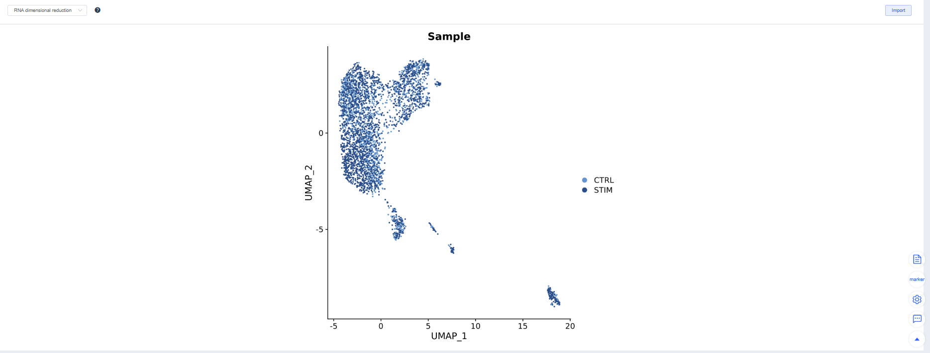
2. After Integration, the system displays the integration results. Adjust parameters and rerun integration as needed. Try multiple methods and choose the one that best suits subsequent analyses.

   

   TIP

   Choosing an integration method:

   • Weak batch effect: merge directly to avoid overcorrection.
   • Moderate batch effect: CCA or RPCA.
   • Pronounced or heterogeneous batches: Harmony is more robust.

   TIP

   Three criteria for evaluating integration quality:

   • Batch mixing: The same cell type mixes evenly across samples on UMAP/TSNE.
   • Biological signal retention: Classic marker gradients and cluster boundaries remain clear, and differential/enrichment results meet expectations.
   • Over/under-correction warnings: Overcorrection flattens differences, while under-correction produces clusters grouped by batch.

Clustering

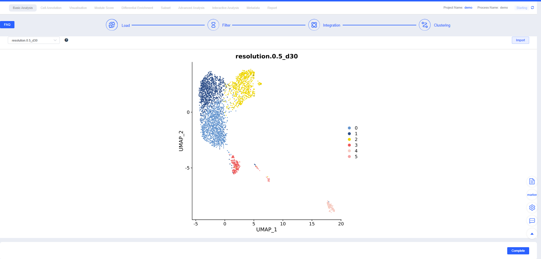
After confirming Integration, proceed with Clustering. You can create clustering results at multiple resolutions; higher resolutions yield more clusters. Additional resolutions can be added in later modules.

TIP

Clustering tuning and troubleshooting:

• Elbow method: Use the PCA elbow point as the starting value for dims; increase it as the cell count grows.
• Subset reclustering: Recluster large categories (e.g., T cells) separately to highlight intra-category heterogeneity. If dims are too low, key heterogeneity may be missed; if too high, overclustering and amplified noise can occur. Optimize based on elbow points and reproducibility.

Complete

If no further adjustments are needed after Clustering, click Complete to jump to the Cell Annotation module and begin downstream single-cell analyses. This step takes some time—please be patient.

"Basic Analysis" is the initial module of the analysis workflow. It performs gene and mitochondrial filtering, batch correction, and clustering to retain high-quality cells for downstream analyses. The steps for creating the workflow and running filtering, integration, and clustering are as follows:

Initial Stage

1. Click Create Process to create a single-cell analysis workflow. Projects typically begin with bulk cluster analysis of selected samples, and you can later choose annotated cell types for subcluster analysis.

2. Enter a "Process Name" and "Description" to help you find and understand the workflow later.

3. Click Select Data to choose the samples for analysis. You can pick pre-integrated multi-sample data or select multiple individual samples for filtering and integration.

NOTE

See Datas for detailed data sources.

4. Click Group to add grouping information (optional). You can also add grouping information in later modules; refer to Plotting Tools for the label feature and Differential Enrichment for grouping functionality.

Filter

1. After you click Start Analysis, the "Charts & Data" section summarizes UMI counts, mitochondrial proportions, and gene expression to provide an overview of sample quality.

NOTE

Metric definitions (scRNA-seq):

• nCount_RNA: Total UMI count per cell, reflecting sequencing depth and transcript abundance
• nFeature_RNA: Number of genes detected per cell, reflecting expression complexity
• Mitochondrial proportion (mito): Percentage of UMIs from mitochondrial genes; elevated levels often indicate apoptosis or damage (increase the allowance slightly for highly metabolic tissues)

2. Expand the panel to view default parameters. You can reference filtering settings reported in published single-cell studies when running Filtering.

TIP

If you selected pre-integrated data, clicking Filtering prompts you to decide whether to skip the filtering and integration steps. Skip them when no parameter adjustments are needed; cancel the skip to rerun filtering and integration when thresholds must be tuned.

IMPORTANT

Filtering strategy recommendations:

• Use MAD-based dynamic thresholds for mt% or reference an upper limit of 10%-20%.
• Identify extreme outliers in nCount_RNA/nFeature_RNA using quantiles or the upper whisker of a boxplot.
• For multi-sample datasets, perform balanced subsampling by cell count to prevent sample size from dominating clustering.
• Relax thresholds for highly metabolic tissues (heart/kidney/liver) or samples rich in immune/granulocyte populations to avoid removing genuine cells.

3. After Filtering, review the post-filtering quality metrics for each sample. You can fine-tune individual samples to maintain consistent overall quality.

   

   CAUTION

   Avoid mechanically "raising cell counts" (for example, loosening lower bounds purely by intuition). If the waterfall plot lacks a clear inflection point, background is high, or low-UMI populations are abnormal, forcing recovery reduces downstream stability. Doublet detection guidelines:

   • Flag high-end tails in nCount_RNA/nFeature_RNA distributions (extreme values on the right).
   • Check for mutually exclusive markers co-expressed or "bridge" cells between two UMAP clusters.
   • In tumor projects, combine CNV evidence.
   • Filter cautiously: remove cells only when multiple lines of evidence agree, and rerun integration and clustering afterward to confirm consistency.

Integration

1. Once QC passes, click Integration. Four integration methods are available; CCA, Harmony, and RPCA perform batch correction across multiple samples.

   

2. After Integration, the system displays the integration results. Adjust parameters and rerun integration as needed. Try multiple methods and choose the one that best suits subsequent analyses.

   

   TIP

   Choosing an integration method:

   • Weak batch effect: merge directly to avoid overcorrection.
   • Moderate batch effect: CCA or RPCA.
   • Pronounced or heterogeneous batches: Harmony is more robust.

   TIP

   Three criteria for evaluating integration quality:

   • Batch mixing: The same cell type mixes evenly across samples on UMAP/TSNE.
   • Biological signal retention: Classic marker gradients and cluster boundaries remain clear, and differential/enrichment results meet expectations.
   • Over/under-correction warnings: Overcorrection flattens differences, while under-correction produces clusters grouped by batch.

Clustering

After confirming Integration, proceed with Clustering. You can create clustering results at multiple resolutions; higher resolutions yield more clusters. Additional resolutions can be added in later modules.

TIP

Clustering tuning and troubleshooting:

• Elbow method: Use the PCA elbow point as the starting value for dims; increase it as the cell count grows.
• Subset reclustering: Recluster large categories (e.g., T cells) separately to highlight intra-category heterogeneity. If dims are too low, key heterogeneity may be missed; if too high, overclustering and amplified noise can occur. Optimize based on elbow points and reproducibility.

Complete

If no further adjustments are needed after Clustering, click Complete to jump to the Cell Annotation module and begin downstream single-cell analyses. This step takes some time—please be patient.

"Basic Analysis" is the initial module of the analysis workflow. It performs gene and mitochondrial filtering, batch correction, and clustering to retain high-quality cells for downstream analyses. The steps for creating the workflow and running filtering, integration, and clustering are as follows:

View more (expand/collapse)

Introduction to Spatial Basic Analysis

Cellular Quality Control

• Cell-level filtering (expression matrix)

  • Use a combination of total UMI count, detected gene count, and mitochondrial proportion, adjusting thresholds to the tissue type.
  • In the SeekSpace workflow, --forceCell and --min_umi are commonly used for the initial pass (for example, extract the top 80,000 UMIs and filter barcodes with UMI < 200 by default). For complex tissues or noisy backgrounds, increase --min_umi appropriately.

• Spatially specific barcode cleaning (critical)

  • Remove invalid spatial barcodes (e.g., short fragments from the expression library or sequencing errors that lack positional information in the HDMI library).
  • Handle spatial barcodes that are duplicated with inconsistent locations: discard those that cannot be uniquely positioned.
  • Eliminate spatial barcode clusters with abnormally high support: divide the chip into grids (such as 30×30-pixel bins), identify suspected delamination/splash hotspots, and remove them (prioritize dropping the spatial barcodes linked to the highest-UMI cell barcode within the bin).
  • Retain only cell barcodes that pass QC and their corresponding valid spatial barcodes.

• Uniqueness check (multi-center cell filtering)

  • Based on the spatial UMI distribution, define a "central bin" and "core region" for each cell, and compute the UMI ratio between the core and secondary centers (≥ 2 indicates a unique center).
  • Remove multi-center cells to reduce ambiguity caused by barcode spillover or nuclear debris.

---

Spatial Mapping

• Coordination of three libraries (SeekSpace example)

  • Expression library: corrects cell barcodes, extracts UMIs, and generates the expression matrix.
  • Spatial library: the Spatai library R2 contains a 32 bp spatial barcode. Extract spatial barcodes from R2 and build the correspondence between cell barcodes and spatial barcodes. Spatial library UMIs (spatial UMIs) represent the expression level of each spatial barcode for each cell barcode.
  • HDMI library: includes 32 bp spatial barcodes and their absolute coordinates; the reads start with the 32 bp spatial barcode followed by coordinate information.

• Correction and registration workflow

  • Barcode level:
    • Correct cell barcodes/UMIs (configure mismatch tolerance such as --skip_misB).
    • Whitelist and correct spatial barcodes, binding them to HDMI coordinates.
  • Image level:
    • Preprocess tissue images (DAPI/HE) by scaling and blurring, then segment tissue regions.
    • If automatic registration is suboptimal, manually align, save parameters (for example, parameters.json), and reuse them in the "realign" workflow to generate consistent background masks and aligned images.

• Establish spatial coordinates and determine cell positions

  • Calculate UMI distributions on grid bins based on the coordinates of spatial barcodes associated with each cell barcode; use the bin with the highest density as the cell center and confirm uniqueness with the core/secondary ratio.
  • Output cell_location.tsv.gz to record cell positions in the chip coordinate system, anchoring the expression matrix in space for visualization overlays.

Refer to SeekSpace Tools for detailed explanations.

The results generated by SeekSpace Tools can be used directly in the cloud platform for downstream analyses.

Initial Stage

1. Click Create Process to create a single-cell analysis workflow. Projects typically begin with bulk cluster analysis of selected samples, and you can later choose annotated cell types for subcluster analysis.

2. Enter a "Process Name" and "Description" to help you find and understand the workflow later.

3. Click Select Data to choose the samples for analysis. You can pick pre-integrated multi-sample data or select multiple individual samples for filtering and integration.

NOTE

See Datas for detailed data sources.

4. Click Group to add grouping information (optional). You can also add grouping information in later modules; refer to Plotting Tools for the label feature and Differential Enrichment for grouping functionality.

Filter

1. After you click Start Analysis, the "Charts & Data" section summarizes UMI counts, mitochondrial proportions, and gene expression to provide an overview of sample quality.

NOTE

Metric definitions (scRNA-seq):

• nCount_RNA: Total UMI count per cell, reflecting sequencing depth and transcript abundance
• nFeature_RNA: Number of genes detected per cell, reflecting expression complexity
• Mitochondrial proportion (mito): Percentage of UMIs from mitochondrial genes; elevated levels often indicate apoptosis or damage (increase the allowance slightly for highly metabolic tissues)

2. Expand the panel to view default parameters. You can reference filtering settings reported in published single-cell studies when running Filtering.

TIP

If you selected pre-integrated data, clicking Filtering prompts you to decide whether to skip the filtering and integration steps. Skip them when no parameter adjustments are needed; cancel the skip to rerun filtering and integration when thresholds must be tuned.

IMPORTANT

Filtering strategy recommendations:

• Use MAD-based dynamic thresholds for mt% or reference an upper limit of 10%-20%.
• Identify extreme outliers in nCount_RNA/nFeature_RNA using quantiles or the upper whisker of a boxplot.
• For multi-sample datasets, perform balanced subsampling by cell count to prevent sample size from dominating clustering.
• Relax thresholds for highly metabolic tissues (heart/kidney/liver) or samples rich in immune/granulocyte populations to avoid removing genuine cells.

3. After Filtering, review the post-filtering quality metrics for each sample. You can fine-tune individual samples to maintain consistent overall quality.

   

   CAUTION

   Avoid mechanically "raising cell counts" (for example, loosening lower bounds purely by intuition). If the waterfall plot lacks a clear inflection point, background is high, or low-UMI populations are abnormal, forcing recovery reduces downstream stability. Doublet detection guidelines:

   • Flag high-end tails in nCount_RNA/nFeature_RNA distributions (extreme values on the right).
   • Check for mutually exclusive markers co-expressed or "bridge" cells between two UMAP clusters.
   • In tumor projects, combine CNV evidence.
   • Filter cautiously: remove cells only when multiple lines of evidence agree, and rerun integration and clustering afterward to confirm consistency.

Integration

1. Once QC passes, click Integration. Four integration methods are available; CCA, Harmony, and RPCA perform batch correction across multiple samples.

   

2. After Integration, the system displays the integration results. Adjust parameters and rerun integration as needed. Try multiple methods and choose the one that best suits subsequent analyses.

   

   TIP

   Choosing an integration method:

   • Weak batch effect: merge directly to avoid overcorrection.
   • Moderate batch effect: CCA or RPCA.
   • Pronounced or heterogeneous batches: Harmony is more robust.

   TIP

   Three criteria for evaluating integration quality:

   • Batch mixing: The same cell type mixes evenly across samples on UMAP/TSNE.
   • Biological signal retention: Classic marker gradients and cluster boundaries remain clear, and differential/enrichment results meet expectations.
   • Over/under-correction warnings: Overcorrection flattens differences, while under-correction produces clusters grouped by batch.

Clustering

After confirming Integration, proceed with Clustering. You can create clustering results at multiple resolutions; higher resolutions yield more clusters. Additional resolutions can be added in later modules.

TIP

Clustering tuning and troubleshooting:

• Elbow method: Use the PCA elbow point as the starting value for dims; increase it as the cell count grows.
• Subset reclustering: Recluster large categories (e.g., T cells) separately to highlight intra-category heterogeneity. If dims are too low, key heterogeneity may be missed; if too high, overclustering and amplified noise can occur. Optimize based on elbow points and reproducibility.

View more (expand/collapse)

Integrating Spatial Clustering with RNA Clustering (Optional)

• Relationship between Banksy and RNA clustering

  • RNA clustering relies solely on gene expression, excelling at distinguishing cell types/states but potentially overlooking spatial continuity and microenvironment cues.
  • Spatial clustering incorporates neighborhood dependence and spatial gradients, revealing functional domains and boundaries, though it may sacrifice some expression resolution.
  • Banksy augments expression features with neighborhood statistics (e.g., neighborhood means/gradients). By adjusting weights, it performs joint clustering to refine RNA cluster boundaries, merge spatially discontinuous pseudo-clusters, or expose spatial functional domains missed by RNA clustering.

• Integration approach (based on the cloud platform workflow)

  • Cloud platform RNA clustering baseline → Import Banksy CSV → Consistency evaluation and differential enrichment
    • Complete standard RNA clustering on the cloud platform to obtain expression-layer baseline labels.
    • Retrieve the Banksy results CSV from Advanced Analysis (e.g., XXX_banksy_colData.csv) and merge it into the workflow meta via "Upload & Merge Meta" (include barcode and avoid column names that conflict with built-in fields).
    • Compare the consistency between RNA baseline and Banksy clusters/spatial domains (NMI/ARI, spatial connectivity/break rate, within-domain expression homogeneity). Use Banksy or the optimized labels as groups for differential expression, enrichment (GO/KEGG/pathways), and spatial visualization.

  TIP

  Why and how to integrate:

  • Joint modeling of "intrinsic expression + spatial microenvironment expression": expression tells you "what it is," space tells you "where it is and what it does."
  • Identify cell subtypes with specific spatial locations to reveal functional subsets restricted to particular regions.
  • Use neighborhood information as supporting evidence to increase confidence: consistent neighborhood expression helps merge pseudo-clusters and suppress noise.
  • Align clustering results with spatial regions more naturally, better matching histological structures and morphological boundaries.

  Banksy is not a replacement for traditional single-cell annotation; it is a powerful enhancement. By injecting critical spatial context into the existing RNA baseline, it elevates our understanding of cell identity from "what it is" to "where it is and what it does."

• Key parameters and practical tips (cloud platform parameter panel)

  • algo: clustering method, supporting leiden, louvain, kmeans, and mclust.
  • Resolution/cluster count:
    • leiden/louvain use resolution (higher values produce more clusters; adjust based on spatial connectivity and marker interpretability).
    • kmeans uses kmeans.centers; mclust uses mclust.G (both specify the number of clusters).
  • lambda: weight between expression and spatial position; 0 disables spatial input. Typical values are 0.1–0.3. Increase slightly for well-structured tissues; decrease for noisy or sparse samples to avoid over-smoothing.
  • Number of principal components: PCs used to build the feature space, default 30. Increase moderately for larger datasets or stronger heterogeneity.

TIP

Tuning suggestions:

• First secure a stable RNA clustering baseline, then grid-search combinations of lambda and resolution (or cluster count) within a narrow range.
• Prefer results balancing higher NMI/ARI with lower spatial break rates; when NMI drops slightly but spatial domains become more continuous and markers align better, favor the Banksy labels.

TIP

Practical advice: fix the RNA resolution to obtain a stable expression baseline, then adjust lambda and k_geom to observe changes in spatial connectivity and NMI. If NMI decreases but the spatial break rate drops markedly and markers form clearer spatial domains, choose the Banksy labels.

• Consistency, interpretability, and deliverables
  • Consistency: report NMI/ARI, spatial break rate, within-domain expression homogeneity, and spatial autocorrelation (e.g., Moran's I).
  • Interpretability: map Banksy clusters to RNA types and verify alignment with domain markers, histological regions, and known structures.
  • Deliverables:
    • Provide a cross-tabulation and side-by-side visualizations (UMAP and spatial coordinates) of "RNA type × spatial domain."
    • Based on differential and enrichment analyses, include spatial heatmaps of significant pathways and representative genes to explain spatial functional differences.

---

• References and further reading

• Banksy resources:

  • Banksy R package GitHub page
  • Banksy original paper (Nature Genetics)

Complete

If no further adjustments are needed after Clustering, click Complete to jump to the Cell Annotation module and begin downstream single-cell analyses. This step takes some time—please be patient.