利用STARsolo+MARVEL来分析单细胞水平的可变剪接
介绍
NOTE
scRNA-seq数据为分析单细胞转录行为带来海量信息,其中不乏工具将单细胞数据转为bulk数据来分析可变剪接,但却失去了单细胞水平上的信息。在此介绍能够在单细胞水平上进行可变剪接的分析流程,是利用STARsolo软件获得Splicing Junction(SJ)信息,并基于MARVEL包来进行剪接事件的量化、差异分析和可视化等。这些单细胞水平的剪接差异对于细胞身份的精细定义、细胞状态的动态转变、疾病特异性机制的揭示以及药物响应的理解至关重要。
IMPORTANT
MARVEL对于基于液滴(Droplet)和平板(Plate)的单细胞数据准备了不同的分析流程,本文档主要介绍基于液滴的单细胞数据分析过程,该过程对寻因全序列、3'、5'数据都适用。其中全序列技术是利用随机引物进行全转录组的随机捕获,得到了更丰富的转录组信息,因此在可变剪接分析上也更有优势。
参考网址:MARVEL
运行准备
IMPORTANT
- 获取"sample_SortedByCoordinate_withTag.bam",该bam是全序列质控分析比对后的bam,并添加了CB/UB的tag
- 请确保运行环境中有STAR(>=2.7.10), samtools, R软件,R中需要提前安装好以下R包:
MARVEL, ggnewscale, ggrepel, reshape2, plyr, stringr, textclean, AnnotationDbi, clusterProfiler, org.Hs.eg.db, gtools, GenomicRanges, IRanges, S4Vectors, wiggleplotr, Matrix, data.table, ggplot2, gridExtra, Seurat, tidyverseCAUTION
3. 准备相应物种的基因组注释文件,文档中以GRCh38作为示例,其中的star索引需要有sjdbList*等文件,生成命令为:
cd path/to/GRCh38/star
STAR \
	--runMode genomeGenerate \
	--genomeDir path/to/GRCh38/star \
	--genomeFastaFiles path/to/GRCh38/fasta/genome.fa \
	--sjdbGTFfile path/to/GRCh38/genes/genes.gtf
STARsolo分析
输入样本名和bam路径,输出路径,在linux环境中执行以下命令:
#!/bin/bash

sample="demo"
outdir="./output"
bam="demo_SortedByCoordinate_withTag.bam"
genome="path/to/GRCh38"

# 创建输出目录
mkdir -p $outdir
cd $outdir
# 对BAM文件进行排序
samtools index $bam
samtools sort -n -@ 20 $bam -o ${sample}_SortedByCoordinate_withTag_resorted.bam

#STAR比对
STAR \
    --runThreadN 8 \
    --genomeDir $genome/star \
    --sjdbGTFfile $genome/genes/genes.gtf \
    --soloType CB_UMI_Simple \
    --readFilesIn ${sample}_SortedByCoordinate_withTag_resorted.bam \
    --readFilesCommand samtools view -F 0x100 -F 0x8 \
    --readFilesType SAM PE \
    --soloCBstart 1 \
    --soloCBlen 17 \
    --soloUMIstart 18 \
    --soloUMIlen 12 \
    --soloCBwhitelist /path/to/seeksoultools/lib/python3.9/site-packages/seeksoultools/mut/barcode/P3CBGB/P3CB.barcode.txt \
    --soloFeatures Gene SJ \
    --outSAMtype None
NOTE
注:参数中--readFilesType PE,是指定了输入的bam是双端比对结果,若用3'数据分析,这里应该调整为--readFilesType SE, 同时不需要进行samtools sort步骤;
参数中通过soloCBwhitelist参数指定barcode白名单,寻因白名单可以从seeksoultools软件中获取。
结果说明
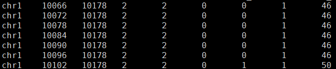
output/Solo.out/SJ/raw/下存放单细胞水平上的SJ信息。barcodes.tsv是barcodes列表,features.tsv是描述的SJ信息,matrix.mtx是对应的UMI数目矩阵。
tree output/Solo.out/SJ/raw/
├── barcodes.tsv
├── features.tsv -> ../../../SJ.out.tab
└── matrix.mtx
features.tsv示例如下,每一行是一个SJ,SJ是指剪接点,对应基因组上一段区域。当这段区域被剪掉时,两边的外显子会连接上,参与形成转录本;当被保留时,这段区域构成转录本的一部分。
Solo.out/Gene/filtered/下输出单细胞的基因表达矩阵
tree output/Solo.out/Gene/filtered/
├── barcodes.tsv
├── features.tsv
└── matrix.mtx
MARVEL分析
接下来,结合STARsolo的输出结果,利用MARVEL工具进行分析。
数据准备
在R环境中执行以下代码
1)首先加载所需R包:
# Load MARVEL package
library(MARVEL)

# Load adjunct packages for selected MARVEL features
  # General data processing, plotting
  library(ggnewscale)
  library(ggrepel)
  library(reshape2)
  library(plyr)
  library(stringr)
  library(textclean)

  # Gene ontology analysis
  library(AnnotationDbi)
  library(clusterProfiler)
  library(org.Hs.eg.db)

  # ad hoc gene candidate gene analysis
  library(gtools)

  # Visualising splice junction location
  library(GenomicRanges)
  library(IRanges)
  library(S4Vectors)
  library(wiggleplotr)

# Load adjunct packages for this tutorial
library(Matrix)
library(data.table)
library(ggplot2)
library(gridExtra)
library(Seurat)
library(tidyverse)
2)读取基因表达信息
TIP
这里直接读取处理好的Seurat Object,获取原始表达数据和标准化后数据。若想要使用STARsolo的基因表达矩阵,请参考MARVEL
# gene info
obj = readRDS("demo_anno.rds")
df.gene.count = obj@assays$RNA$counts
df.gene.norm = obj@assays$RNA$data
df.gene.norm.pheno = obj@meta.data %>% mutate(cell.id = rownames(.))
df.gene.count.pheno = df.gene.norm.pheno
df.gene.norm.feature = data.frame(gene_short_name = rownames(obj))
df.gene.count.feature = df.gene.norm.feature
3)读取SJ矩阵,从STARsolo输出结果中获取。
df.sj.count = readMM('output/Solo.out/SJ/raw/matrix.mtx')
cell_name = read.table('output/Solo.out/SJ/raw/barcodes.tsv',
                       header=F, sep='\t')
df.sj.count.feature = read.table('output/Solo.out/SJ/raw/features.tsv',
                      sep="\t", header=FALSE, stringsAsFactors=FALSE)[,1:3]

df.sj.count.feature$coord.intron = paste0(df.sj.count.feature$V1,
    ':',df.sj.count.feature$V2,
    ':',df.sj.count.feature$V3)
colnames(df.sj.count) = cell_name$V1
rownames(df.sj.count) = df.sj.count.feature$coord.intron
df.sj.count = df.sj.count[,colnames(obj)]
df.sj.count[1:3,1:3]

df.sj.count.pheno = data.frame(cell.id = colnames(df.sj.count))
4)读取细胞在降维图上的坐标和gtf文件,为后续画图做准备。
df.coord = Embeddings(obj, reduction =  'umap') %>% as.data.frame()
colnames(df.coord) = c('x','y')
df.coord = df.coord %>% rownames_to_column('cell.id')

gtf <- as.data.frame(fread("path/to/GRCh38/genes/genes.gtf",
                           sep="\t", header=FALSE, stringsAsFactors=FALSE))
执行成功后,MARVEL分析所需要的数据已经准备好了。
构建MARVEL对象
IMPORTANT
接下来,可以构建MARVEL对象,并进行预处理:
marvel <- CreateMarvelObject.10x(gene.norm.matrix=df.gene.norm,
                                 gene.norm.pheno=df.gene.norm.pheno,
                                 gene.norm.feature=df.gene.norm.feature,
                                 gene.count.matrix=df.gene.count,
                                 gene.count.pheno=df.gene.count.pheno,
                                 gene.count.feature=df.gene.count.feature,
                                 sj.count.matrix=df.sj.count,
                                 sj.count.pheno=df.sj.count.pheno,
                                 sj.count.feature=df.sj.count.feature,
                                 pca=df.coord,
                                 gtf=gtf
                                 )

marvel <- AnnotateGenes.10x(MarvelObject=marvel)
marvel <- AnnotateSJ.10x(MarvelObject=marvel)
marvel <- ValidateSJ.10x(MarvelObject=marvel)
marvel <- FilterGenes.10x(MarvelObject=marvel,
                          gene.type=c("protein_coding", "lncRNA"))
marvel <- CheckAlignment.10x(MarvelObject=marvel)
查询SJ的meta信息:
head(marvel$sj.metadata)保存对象:
saveRDS(marvel,file="demo_marvel.rds")下游分析与可视化
1)SJ在细胞群间的差异分析
TIP
以比较Tcell和Myeloid之间的差异SJ为例:
meta_=marvel$sample.metadata
cell.ids.1 <- meta_$cell.id[meta_$celltype == "Tcell"]
cell.ids.2 <- meta_$cell.id[meta_$celltype == "Myeloid"]

marvel_10X_T <- CompareValues.SJ.10x(MarvelObject=marvel,
                               cell.group.g1=cell.ids.1,
                               cell.group.g2=cell.ids.2,
                               min.pct.cells.genes=10,
                               min.pct.cells.sj=10,
                               min.gene.norm=1.0,
                               seed=1,
                               n.iterations=100,
                               downsample=TRUE,
                               show.progress=FALSE
                               )
head(marvel$DE$SJ$Table)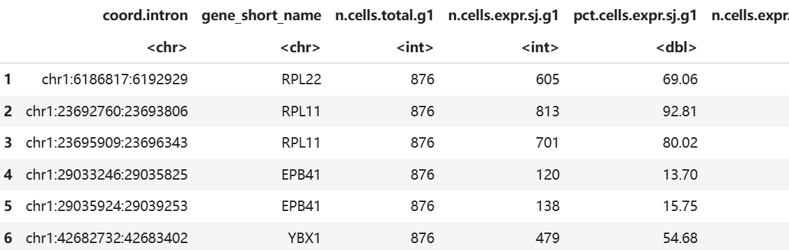
表格中包含SJ的差异水平,PSI等信息。PSI是指Percent Spliced in,描述该区域是倾向于被保留还是被剪掉,值越大,说明被保留。
| coord.intron | SJ |
|---|---|
| gene_short_name | 可变剪接所属基因 |
| n.cells.total.g1 | group1里的细胞数 |
| n.cells.expr.sj.g1 | group1里表达该SJ的细胞数 |
| pct.cells.expr.sj.g1 | group1里表达该SJ的细胞比例 |
| n.cells.expr.gene.g1 | group1里表达该基因的细胞数 |
| pct.cells.expr.gene.g1 | group1里表达该基因的细胞比例 |
| sj.count.total.g1 | group1的reads数 |
| gene.count.total.g1 | group1里该基因表达数目 |
| psi.g1 | group1的PSI值 |
| n.cells.total.g2 | group2里的细胞数 |
| n.cells.expr.sj.g2 | group2里表达该SJ的细胞数 |
| pct.cells.expr.sj.g2 | group2里表达该SJ的细胞比例 |
| n.cells.expr.gene.g2 | group2里表达该基因的细胞数 |
| pct.cells.expr.gene.g2 | group2里表达该基因的细胞比例 |
| sj.count.total.g2 | group2的reads数 |
| gene.count.total.g2 | group2的基因表达数目 |
| psi.g2 | group2的PSI值 |
| log2fc | CompareValues.SJ.10x计算出来的log-Fold-change |
| delta | PSI差值 |
2)可视化:依次展示细胞分组,基因表达,该基因某个SJ的PSI
# compare list
cell.ids.1 <- meta_$cell.id[meta_$celltype == "Tcell" & meta_$Sample == "cancer"]
cell.ids.2 <- meta_$cell.id[meta_$celltype == "Tcell" & meta_$Sample == "normal"]
cell.group.list <- list("cancer"=cell.ids.1,
                         "normal"=cell.ids.2)

# Plot cell groups
marvel <- PlotValues.PCA.CellGroup.10x(MarvelObject=marvel_fmarvelast_T,
                                       cell.group.list=cell.group.list,
                                       legendtitle="Cell group",
                                       type="tsne"
                                       )
plot_group <- marvel$adhocPlot$PCA$CellGroup

# Plot gene expression
marvel <- PlotValues.PCA.Gene.10x(MarvelObject=marvel,
                                  gene_short_name="PTPRC",
                                  color.gradient=c("grey","cyan","green","yellow","red"),
                                  type="tsne"
                                  )
plot_gene <- marvel$adhocPlot$PCA$Gene

# Plot PSI
marvel <- PlotValues.PCA.PSI.10x(MarvelObject=marvel,
                                 coord.intron="chr1:198742368:198744053",
                                 min.gene.count=3,
                                 log2.transform=FALSE,
                                 color.gradient=c("grey","cyan","green","yellow","red"),
                                 type="tsne"
                                 )
plot_sj <- marvel$adhocPlot$PCA$PSI

# Arrange and view plots
grid.arrange(plot_group, plot_gene, plot_sj, nrow=1)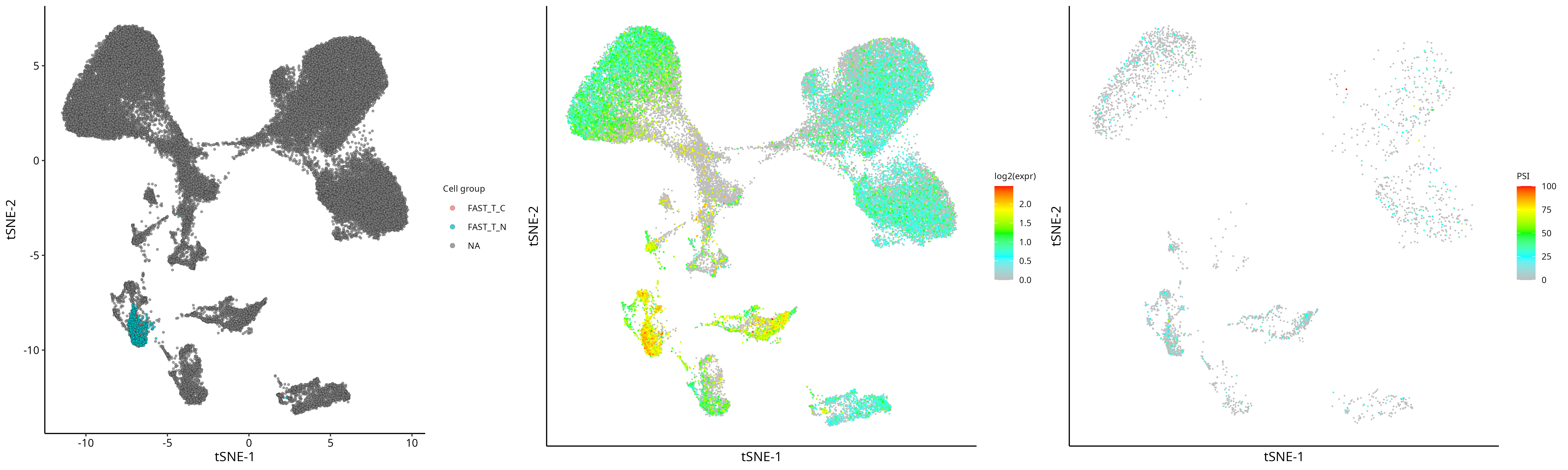
3)可视化:比较某个基因在细胞群间的表达水平和其所有SJ的表达水平
以CD53基因为例:
sample.metadata=marvel$sample.metadata

SJ_PSI_list = list()
all_celltype=unique(sample.metadata$celltype)

#get diff SJ for all celltypes
for(cluster_i in all_celltype) {
    cell.ids.1 <- sample.metadata[sample.metadata$celltype == cluster_i, "cell.id"]
    cell.ids.2 <- sample.metadata[sample.metadata$celltype != cluster_i, "cell.id"]

    tmp <- CompareValues.SJ.10x(MarvelObject=marvel,
                               cell.group.g1=cell.ids.1,
                               cell.group.g2=cell.ids.2,
                               min.pct.cells.genes=10,
                               min.pct.cells.sj=10,
                               min.gene.norm=1.0,
                               seed=1,
                               n.iterations=100,
                               downsample=TRUE,
                               show.progress=FALSE
                               )

    res=tmp$DE$SJ$Table
    res$cluster=cluster_i
    res$vs=paste0(cluster_i,"_vs_","others")
    SJ_PSI_list[[cluster_i]]=res
    }
SJ_diff_all=Reduce(rbind,SJ_PSI_list)

#add info
SJ_diff_all$name=paste0(SJ_diff_all$coord.intron,"_",SJ_diff_all$cluster)
SJ_diff_all$cluster=factor(SJ_diff_all$cluster,levels=all_celltype)
SJ_diff_all$name=paste0(SJ_diff_all$coord.intron,"(",SJ_diff_all$gene_short_name,")")
head(SJ_diff_all)

#select CD53 for plot
plot_data=SJ_diff_all[SJ_diff_all$gene_short_name == "CD53",
               c("cluster","coord.intron","name","psi.g1","pct.cells.expr.sj.g1")]
colnames(plot_data)=c("cluster","coord.intron","name","PSI","pct.cell")
plot_data$cluster=as.character(plot_data$cluster)
plot_data$cluster=factor(plot_data$cluster,levels=all_celltype)
plot_data <- plot_data[order(plot_data$coord.intron), ]

p = ggplot(plot_data, aes(x = cluster, y = name)) +
  geom_point(aes(size = pct.cell, color = PSI)) +
  theme_minimal(base_size = 15) +
  scale_color_gradientn(
    colors = c("white",'#FF8247'),
    na.value = "white"
  ) +
  theme(
    panel.grid = element_blank(),
    axis.title = element_blank(),
    plot.title = element_text(hjust = 1, size = 12),
    panel.border = element_rect(colour = "grey", fill = NA, linewidth = 0.5)
  )
p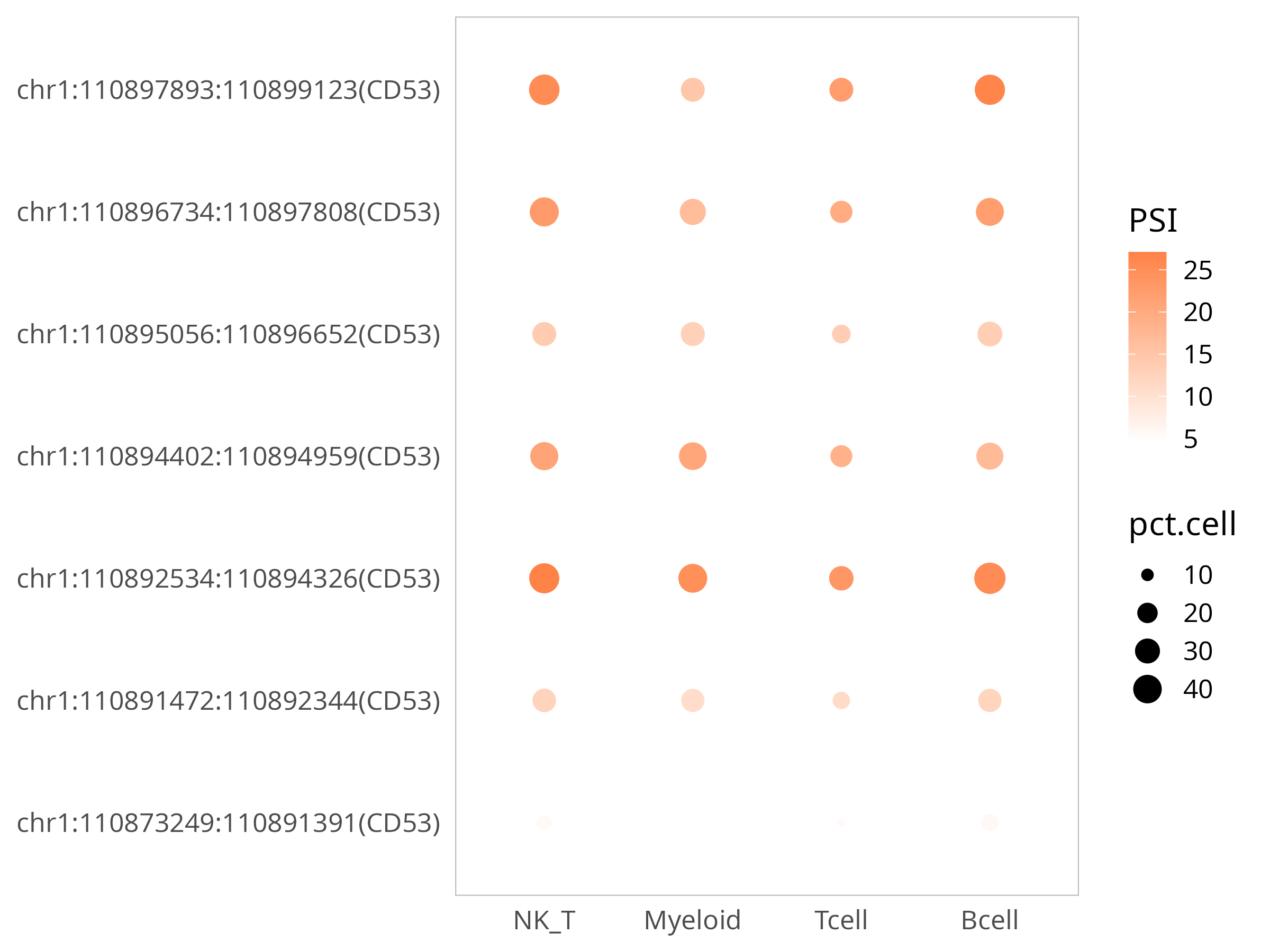
NOTE
上方气泡图是展示该基因检测到的所有SJ的表达水平,PSI是表示该SJ被保留的程度,越大越被保留;pct表示细胞表达比例;该图可以直观了解基因不同区段在细胞群上的表达差异。
总结
本文档总结了利用STARsolo和MARVEL流程来分析单细胞的可变剪接内容,内容有限,可以根据实际案例或相关文章进行拓展。