Analysis of Alternative Splicing at Single-Cell Level Using STARsolo and MARVEL
Introduction
NOTE
scRNA-seq data provides massive information for analyzing transcriptional behavior at single-cell resolution. While many tools convert single-cell data to bulk data for alternative splicing analysis, this approach loses single-cell level information. Here we introduce an analysis pipeline for alternative splicing at single-cell level, utilizing STARsolo software to obtain Splicing Junction (SJ) information, and MARVEL package for splicing event quantification, differential analysis, and visualization. These single-cell level splicing differences are crucial for fine definition of cell identity, dynamic transitions of cell states, revelation of disease-specific mechanisms, and understanding of drug responses.
IMPORTANT
MARVEL provides different analysis pipelines for droplet-based and plate-based single-cell data. This document mainly introduces the droplet-based single-cell data analysis process, which is applicable to FAST, 3', and 5' data. Among these, FAST technology uses random primers for whole transcriptome random capture, providing richer transcriptome information and thus having advantages in alternative splicing analysis.
Reference website: MARVEL
Preparation
IMPORTANT
Obtain "sample_SortedByCoordinate_withTag.bam", which is the bam file after quality control and alignment of FAST data, with CB/UB tags added;
Ensure the running environment has STAR (>=2.7.10), samtools, R software, and the following R packages installed:
MARVEL, ggnewscale, ggrepel, reshape2, plyr, stringr, textclean, AnnotationDbi, clusterProfiler, org.Hs.eg.db, gtools, GenomicRanges, IRanges, S4Vectors, wiggleplotr, Matrix, data.table, ggplot2, gridExtra, Seurat, tidyverseCAUTION
3) Prepare genome annotation files for the corresponding species. This document uses GRCh38 as an example. The star index needs to have sjdbList* files, generated with the following command:
cd path/to/GRCh38/star
STAR \
    --runMode genomeGenerate \
    --genomeDir path/to/GRCh38/star \
    --genomeFastaFiles path/to/GRCh38/fasta/genome.fa \
    --sjdbGTFfile path/to/GRCh38/genes/genes.gtf
STARsolo Analysis
Input sample name and bam path, output path, execute the following command in Linux environment:
#!/bin/bash

sample="demo"
outdir="./output"
bam="demo_SortedByCoordinate_withTag.bam"
genome="path/to/GRCh38"

# Create output directory
mkdir -p $outdir
cd $outdir
# Sort BAM file
samtools index $bam
samtools sort -n -@ 20 $bam -o ${sample}_SortedByCoordinate_withTag_resorted.bam

#STAR alignment
STAR \
    --runThreadN 8 \
    --genomeDir $genome/star \
    --sjdbGTFfile $genome/genes/genes.gtf \
    --soloType CB_UMI_Simple \
    --readFilesIn ${sample}_SortedByCoordinate_withTag_resorted.bam \
    --readFilesCommand samtools view -F 0x100 -F 0x8 \
    --readFilesType SAM PE \
    --soloCBstart 1 \
    --soloCBlen 17 \
    --soloUMIstart 18 \
    --soloUMIlen 12 \
    --soloCBwhitelist /path/to/seeksoultools/lib/python3.9/site-packages/seeksoultools/mut/barcode/P3CBGB/P3CB.barcode.txt \
    --soloFeatures Gene SJ \
    --outSAMtype None
NOTE
Note: The parameter --readFilesType PE specifies that the input bam is paired-end alignment result. For 3' data analysis, this should be changed to --readFilesType SE, and the samtools sort step is not necessary;
The barcode whitelist is specified through the soloCBwhitelist parameter, and the whitelist can be obtained from the seeksoultools software.
Results Description
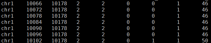
SJ information at single-cell level is stored in output/Solo.out/SJ/raw/. barcodes.tsv is the barcodes list, features.tsv describes SJ information, and matrix.mtx is the corresponding UMI count matrix.
tree output/Solo.out/SJ/raw/
├── barcodes.tsv
├── features.tsv -> ../../../SJ.out.tab
└── matrix.mtx
Example of features.tsv is shown below. Each row represents an SJ, which corresponds to a genomic region. When this region is spliced out, the exons on both sides will connect to form a transcript; when retained, this region becomes part of the transcript.
Single-cell gene expression matrix is output in Solo.out/Gene/filtered/
tree output/Solo.out/Gene/filtered/
├── barcodes.tsv
├── features.tsv
└── matrix.mtx
MARVEL Analysis
Next, we use MARVEL tool to analyze the output results from STARsolo.
Data Preparation
Execute the following code in R environment
1) First load required R packages:
# Load MARVEL package
library(MARVEL)

# Load adjunct packages for selected MARVEL features
  # General data processing, plotting
  library(ggnewscale)
  library(ggrepel)
  library(reshape2)
  library(plyr)
  library(stringr)
  library(textclean)

  # Gene ontology analysis
  library(AnnotationDbi)
  library(clusterProfiler)
  library(org.Hs.eg.db)

  # ad hoc gene candidate gene analysis
  library(gtools)

  # Visualising splice junction location
  library(GenomicRanges)
  library(IRanges)
  library(S4Vectors)
  library(wiggleplotr)

# Load adjunct packages for this tutorial
library(Matrix)
library(data.table)
library(ggplot2)
library(gridExtra)
library(Seurat)
library(tidyverse)
2) Read gene expression information
TIP
Here we directly read the processed Seurat Object to obtain raw expression data and normalized data. If you want to use STARsolo's gene expression matrix, please refer to MARVEL
# gene info
obj = readRDS("demo_anno.rds")
df.gene.count = obj@assays$RNA$counts
df.gene.norm = obj@assays$RNA$data
df.gene.norm.pheno = obj@meta.data %>% mutate(cell.id = rownames(.))
df.gene.count.pheno = df.gene.norm.pheno
df.gene.norm.feature = data.frame(gene_short_name = rownames(obj))
df.gene.count.feature = df.gene.norm.feature
3) Read SJ matrix from STARsolo output results
df.sj.count = readMM('output/Solo.out/SJ/raw/matrix.mtx')
cell_name = read.table('output/Solo.out/SJ/raw/barcodes.tsv',
                       header=F, sep='\t')
df.sj.count.feature = read.table('output/Solo.out/SJ/raw/features.tsv',
                      sep="\t", header=FALSE, stringsAsFactors=FALSE)[,1:3]

df.sj.count.feature$coord.intron = paste0(df.sj.count.feature$V1,
    ':',df.sj.count.feature$V2,
    ':',df.sj.count.feature$V3)
colnames(df.sj.count) = cell_name$V1
rownames(df.sj.count) = df.sj.count.feature$coord.intron
df.sj.count = df.sj.count[,colnames(obj)]
df.sj.count[1:3,1:3]

df.sj.count.pheno = data.frame(cell.id = colnames(df.sj.count))
4) Read cell coordinates in dimensionality reduction plot and gtf file for subsequent plotting
df.coord = Embeddings(obj, reduction =  'umap') %>% as.data.frame()
colnames(df.coord) = c('x','y')
df.coord = df.coord %>% rownames_to_column('cell.id')

gtf <- as.data.frame(fread("path/to/GRCh38/genes/genes.gtf",
                           sep="\t", header=FALSE, stringsAsFactors=FALSE))
After successful execution, the data needed for MARVEL analysis is ready.
Create MARVEL Object
IMPORTANT
Next, we can create the MARVEL object and perform preprocessing:
marvel <- CreateMarvelObject.10x(gene.norm.matrix=df.gene.norm,
                                 gene.norm.pheno=df.gene.norm.pheno,
                                 gene.norm.feature=df.gene.norm.feature,
                                 gene.count.matrix=df.gene.count,
                                 gene.count.pheno=df.gene.count.pheno,
                                 gene.count.feature=df.gene.count.feature,
                                 sj.count.matrix=df.sj.count,
                                 sj.count.pheno=df.sj.count.pheno,
                                 sj.count.feature=df.sj.count.feature,
                                 pca=df.coord,
                                 gtf=gtf
                                 )

marvel <- AnnotateGenes.10x(MarvelObject=marvel)
marvel <- AnnotateSJ.10x(MarvelObject=marvel)
marvel <- ValidateSJ.10x(MarvelObject=marvel)
marvel <- FilterGenes.10x(MarvelObject=marvel,
                          gene.type=c("protein_coding", "lncRNA"))
marvel <- CheckAlignment.10x(MarvelObject=marvel)
Query SJ meta information:
head(marvel$sj.metadata)Save object:
saveRDS(marvel,file="demo_marvel.rds")Downstream Analysis and Visualization
1) Differential Analysis of SJ between Cell Groups
TIP
Taking comparison of differential SJ between Tcell and Myeloid as an example:
meta_=marvel$sample.metadata
cell.ids.1 <- meta_$cell.id[meta_$celltype == "Tcell"]
cell.ids.2 <- meta_$cell.id[meta_$celltype == "Myeloid"]

marvel_10X_T <- CompareValues.SJ.10x(MarvelObject=marvel,
                               cell.group.g1=cell.ids.1,
                               cell.group.g2=cell.ids.2,
                               min.pct.cells.genes=10,
                               min.pct.cells.sj=10,
                               min.gene.norm=1.0,
                               seed=1,
                               n.iterations=100,
                               downsample=TRUE,
                               show.progress=FALSE
                               )
head(marvel$DE$SJ$Table)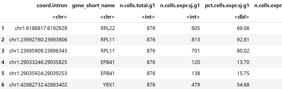
The table contains SJ differential levels, PSI and other information. PSI refers to Percent Spliced in, describing whether the region tends to be retained or spliced out. The larger the value, the more likely it is to be retained.
| coord.intron | SJ |
|---|---|
| gene_short_name | Gene containing the alternative splicing |
| n.cells.total.g1 | Number of cells in group1 |
| n.cells.expr.sj.g1 | Number of cells expressing this SJ in group1 |
| pct.cells.expr.sj.g1 | Percentage of cells expressing this SJ in group1 |
| n.cells.expr.gene.g1 | Number of cells expressing this gene in group1 |
| pct.cells.expr.gene.g1 | Percentage of cells expressing this gene in group1 |
| sj.count.total.g1 | Read count in group1 |
| gene.count.total.g1 | Gene expression count in group1 |
| psi.g1 | PSI value in group1 |
| n.cells.total.g2 | Number of cells in group2 |
| n.cells.expr.sj.g2 | Number of cells expressing this SJ in group2 |
| pct.cells.expr.sj.g2 | Percentage of cells expressing this SJ in group2 |
| n.cells.expr.gene.g2 | Number of cells expressing this gene in group2 |
| pct.cells.expr.gene.g2 | Percentage of cells expressing this gene in group2 |
| sj.count.total.g2 | Read count in group2 |
| gene.count.total.g2 | Gene expression count in group2 |
| psi.g2 | PSI value in group2 |
| log2fc | log-Fold-change calculated by CompareValues.SJ.10x |
| delta | PSI difference |
2) Visualization: Display cell grouping, gene expression, and PSI of a specific SJ of the gene
# compare list
cell.ids.1 <- meta_$cell.id[meta_$celltype == "Tcell" & meta_$Sample == "cancer"]
cell.ids.2 <- meta_$cell.id[meta_$celltype == "Tcell" & meta_$Sample == "normal"]
cell.group.list <- list("cancer"=cell.ids.1,
                         "normal"=cell.ids.2)

# Plot cell groups
marvel <- PlotValues.PCA.CellGroup.10x(MarvelObject=marvel_fmarvelast_T,
                                       cell.group.list=cell.group.list,
                                       legendtitle="Cell group",
                                       type="tsne"
                                       )
plot_group <- marvel$adhocPlot$PCA$CellGroup

# Plot gene expression
marvel <- PlotValues.PCA.Gene.10x(MarvelObject=marvel,
                                  gene_short_name="PTPRC",
                                  color.gradient=c("grey","cyan","green","yellow","red"),
                                  type="tsne"
                                  )
plot_gene <- marvel$adhocPlot$PCA$Gene

# Plot PSI
marvel <- PlotValues.PCA.PSI.10x(MarvelObject=marvel,
                                 coord.intron="chr1:198742368:198744053",
                                 min.gene.count=3,
                                 log2.transform=FALSE,
                                 color.gradient=c("grey","cyan","green","yellow","red"),
                                 type="tsne"
                                 )
plot_sj <- marvel$adhocPlot$PCA$PSI

# Arrange and view plots
grid.arrange(plot_group, plot_gene, plot_sj, nrow=1)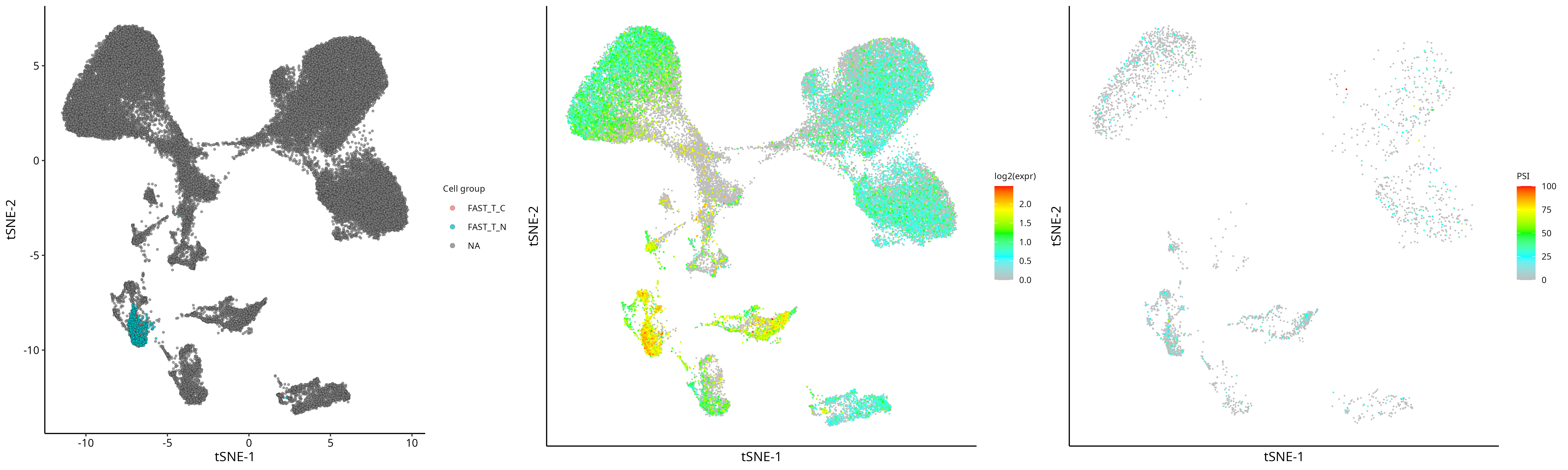
3) Visualization: Compare expression levels of a gene and all its SJs between cell groups
Taking CD53 gene as an example:
sample.metadata=marvel$sample.metadata

SJ_PSI_list = list()
all_celltype=unique(sample.metadata$celltype)

#get diff SJ for all celltypes
for(cluster_i in all_celltype) {
    cell.ids.1 <- sample.metadata[sample.metadata$celltype == cluster_i, "cell.id"]
    cell.ids.2 <- sample.metadata[sample.metadata$celltype != cluster_i, "cell.id"]

    tmp <- CompareValues.SJ.10x(MarvelObject=marvel,
                               cell.group.g1=cell.ids.1,
                               cell.group.g2=cell.ids.2,
                               min.pct.cells.genes=10,
                               min.pct.cells.sj=10,
                               min.gene.norm=1.0,
                               seed=1,
                               n.iterations=100,
                               downsample=TRUE,
                               show.progress=FALSE
                               )

    res=tmp$DE$SJ$Table
    res$cluster=cluster_i
    res$vs=paste0(cluster_i,"_vs_","others")
    SJ_PSI_list[[cluster_i]]=res
    }
SJ_diff_all=Reduce(rbind,SJ_PSI_list)

#add info
SJ_diff_all$name=paste0(SJ_diff_all$coord.intron,"_",SJ_diff_all$cluster)
SJ_diff_all$cluster=factor(SJ_diff_all$cluster,levels=all_celltype)
SJ_diff_all$name=paste0(SJ_diff_all$coord.intron,"(",SJ_diff_all$gene_short_name,")")
head(SJ_diff_all)

#select CD53 for plot
plot_data=SJ_diff_all[SJ_diff_all$gene_short_name == "CD53",
               c("cluster","coord.intron","name","psi.g1","pct.cells.expr.sj.g1")]
colnames(plot_data)=c("cluster","coord.intron","name","PSI","pct.cell")
plot_data$cluster=as.character(plot_data$cluster)
plot_data$cluster=factor(plot_data$cluster,levels=all_celltype)
plot_data <- plot_data[order(plot_data$coord.intron), ]

p = ggplot(plot_data, aes(x = cluster, y = name)) +
  geom_point(aes(size = pct.cell, color = PSI)) +
  theme_minimal(base_size = 15) +
  scale_color_gradientn(
    colors = c("white",'#FF8247'),
    na.value = "white"
  ) +
  theme(
    panel.grid = element_blank(),
    axis.title = element_blank(),
    plot.title = element_text(hjust = 1, size = 12),
    panel.border = element_rect(colour = "grey", fill = NA, linewidth = 0.5)
  )
p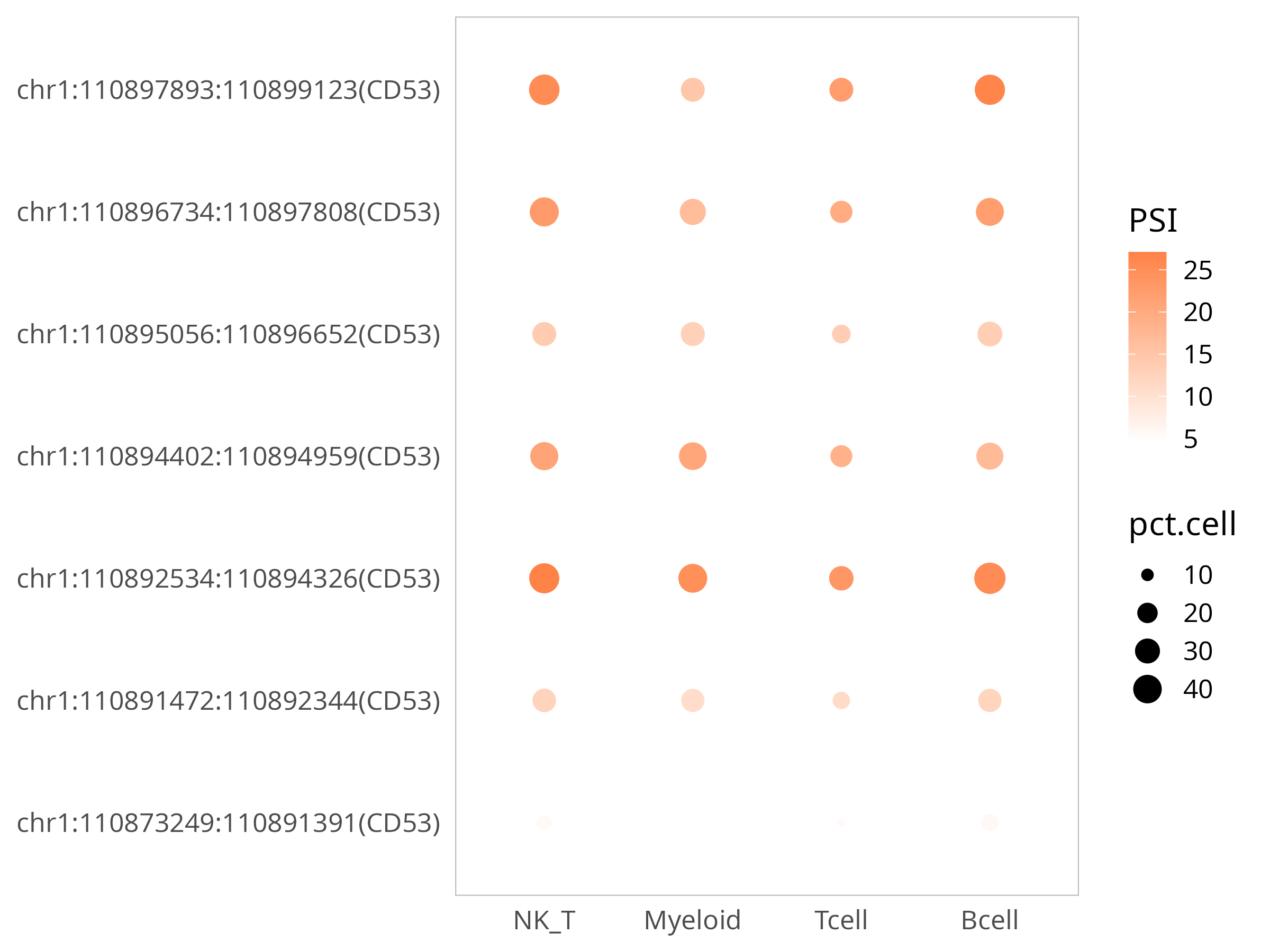
NOTE
The bubble plot above shows the expression levels of all SJs detected for this gene. PSI indicates the degree to which the SJ is retained, with larger values indicating more retention; pct represents the percentage of cells expressing it; this plot can intuitively understand the expression differences of different gene segments across cell groups.
Summary
This document summarizes the process of analyzing alternative splicing at single-cell level using STARsolo and MARVEL pipeline. The content is limited and can be expanded based on actual cases or related literature.